Beyond LLMS
CLIP, OpenCLIP, and SigLIP: Contrastive Language-Image Pretraining
Radford et al. 2021 (CLIP) trained two encoders, one for images and one for text, with a symmetric InfoNCE objective on 400M web pairs. The result was a shared embedding space that powers zero-shot classification, retrieval, and serves as the visual backbone of every modern vision-language model. This page covers the contrastive objective as a mutual-information bound, the OpenCLIP scaling laws (Cherti et al. 2023), the SigLIP pairwise-sigmoid alternative (Zhai et al. 2023), the modality gap (Liang et al. 2022), and the practical pipeline from training corpus to LLaVA-style VLM backbone.
Prerequisites
Why This Matters
Before CLIP (Radford et al., 2021), using a vision model on a new task meant collecting labeled images and fine-tuning a supervised classifier. CLIP replaced the classifier with a shared embedding space: one image encoder and one text encoder, trained jointly on 400 million web image-caption pairs so that matching pairs land near each other in and non-matching pairs land far apart. The result is zero-shot classification by similarity: you describe the categories in words, encode the descriptions, and pick the nearest text vector to the image vector. No labeled data for the target task, no fine-tuning.
Hide overviewShow overview
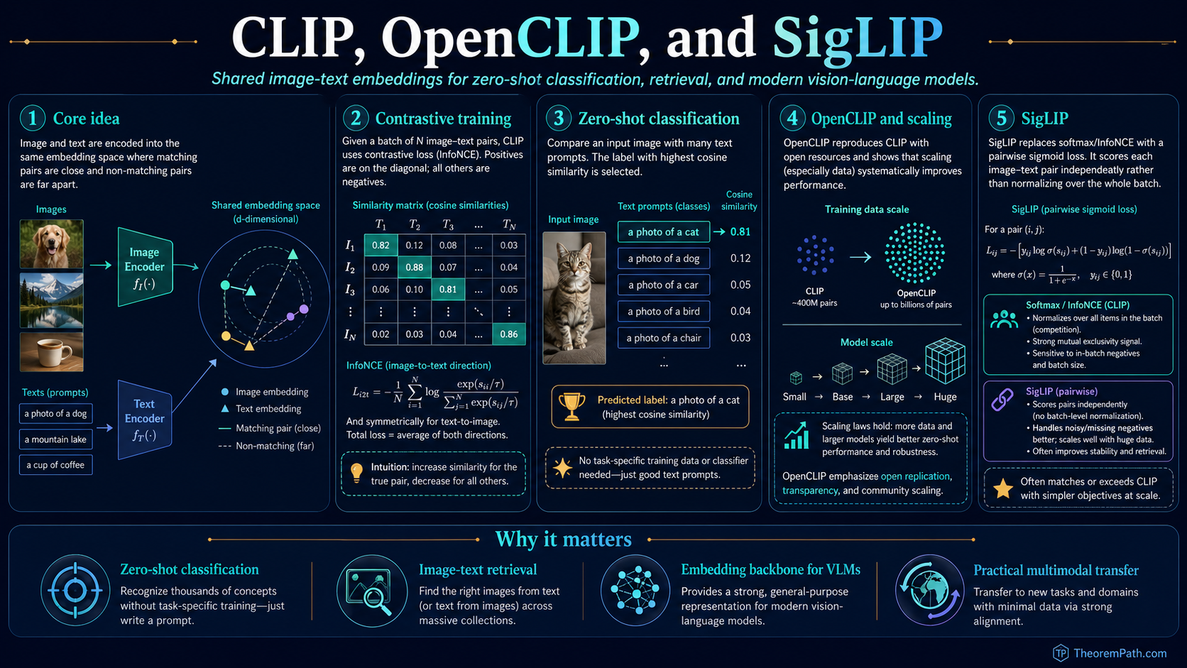
InfoNCE (row-wise softmax) vs. SigLIP (per-cell sigmoid) on an N=8 batch
This is the same shift that happened in NLP with large language models: from task-specific supervised models to general-purpose pretrained models that adapt via natural-language prompts. CLIP brought it to vision and gave every later vision-language model a usable visual backbone. Modern VLMs (LLaVA, BLIP-2, Qwen-VL, InternVL, Molmo) use a frozen or lightly finetuned CLIP-style encoder as their image input pathway. Image-conditioned diffusion models (Stable Diffusion 1.x/2.x/SDXL/SD3) use a CLIP text encoder to condition the noise-prediction network. The frontier multimodal pipeline is built on top of contrastive image-text alignment.
The page covers four things in order: the contrastive objective and its mutual-information interpretation, the OpenCLIP reproductions and scaling laws, the SigLIP pairwise-sigmoid alternative that has displaced softmax NCE in many recent systems, and the geometric properties (modality gap, hubness, prompt sensitivity) that constrain how the embeddings can be used.
Mental Model
Two encoders run in parallel:
- Image encoder (a Vision Transformer in modern variants; a ResNet in the original 2021 paper).
- Text encoder (a Transformer with byte-pair tokenization).
Both produce -normalized embeddings of the same dimension . The similarity between an image and a text is the dot product of their unit-vector embeddings, which equals their cosine similarity: . Training pulls matching pairs toward and pushes non-matching pairs toward zero or below.
At inference, classification is a nearest-neighbor lookup in this embedding space. To classify an image into one of categories, build a text prompt "a photo of a [class name]" for each category, encode all prompts, encode the image, and pick the prompt with the highest cosine similarity. The model has never seen labels for the target task; the labels live entirely in natural language and the encoders' shared geometry handles the rest.
| Component | Role | Frontier replacement |
|---|---|---|
| Image encoder | maps image to unit sphere | ViT-L/14, ViT-H/14, ViT-G/14, EVA-02, SigLIP-SoViT |
| Text encoder | maps text to unit sphere | original CLIP transformer; SigLIP T5-style; OpenCLIP variants |
| Loss | symmetric InfoNCE over batch | SigLIP pairwise sigmoid (no batch-wide softmax) |
| Pretraining data | 400M WebImageText pairs (closed) | LAION-2B, DataComp-1B, COYO-700M (open) |
Formal Setup
CLIP Dual Encoder
A CLIP-style model is a pair of encoders mapping images and text into the unit sphere . The image encoder is a ViT or ResNet trunk followed by a linear projection and normalization; the text encoder is a Transformer over BPE tokens with the end-of-text token's hidden state projected and normalized identically.
The bilinear similarity is
is a cosine similarity bounded in and the training objective scales it by a learned temperature parameter.
Zero-Shot Classification with CLIP
Given an image and class names , build text prompts "a photo of a " (or an ensemble of templates). The predicted class is . No task-specific training data is needed; the only "training" is the choice of prompt template.
The CLIP-400M dataset (the original closed corpus from Radford et al.) consists of 400 million (image, caption) pairs scraped from the public web. Each pair is an image and its associated alt text or caption. The data are noisy, diverse, and massive. The scale and breadth of the corpus are what give CLIP its generalization ability; ablations in the original paper and in OpenCLIP show that data quantity beats data cleanliness within several orders of magnitude.
OpenCLIP is the open-source reproduction of CLIP by LAION. It ships models trained on different corpora (LAION-400M, LAION-2B, DataComp-1B) with a range of architectures (ViT-B/32 through ViT-G/14) and training recipes, and it is the substrate for the Cherti et al. 2023 scaling-laws paper that established quantitative compute / data / parameter exponents for the contrastive setup.
The Contrastive Objective
CLIP Symmetric Contrastive Loss
Statement
Given a batch of pairs, let and be the normalized embeddings. With learned temperature , the CLIP loss is the symmetric cross-entropy over the scaled-similarity matrix:
The first term treats each image as a query and finds its matching text among candidates; the second is the reverse. Diagonal entries of the similarity matrix are positives; off-diagonal entries are in-batch negatives. The temperature is initialized to in the original parameterization and learned end-to-end (with a clamp to prevent divergence).
Intuition
Each image should be most similar to its own caption and dissimilar to all other captions in the batch, and symmetrically each caption should be most similar to its own image. With batch size each positive pair is contrasted against negatives, providing a rich signal that forces the encoders to learn fine-grained semantic distinctions. The temperature controls how peaked the similarity distribution is: large produces a sharp softmax that punishes near-misses heavily, small produces a soft distribution that gives gradient mass to many candidates.
Proof Sketch
The loss is the standard multi-class cross-entropy with classes (one per batch slot). By the standard analysis of softmax cross-entropy, the gradient on from the image-to-text term is where is the softmax-normalized probability of pair . This pushes toward (the positive) and away from a probability-weighted average of all negatives. Symmetric treatment ensures both encoders learn compatible representations.
Why It Matters
This single objective is why CLIP generalizes to unseen tasks. The combination of (a) a contrastive loss that scales with batch size, (b) a learned temperature that adapts to embedding quality, and (c) hundreds of millions of diverse pairs produces an embedding space where semantic similarity aligns with geometric proximity. Any concept expressible in text (including concepts not in any predefined label set) can be matched to images by computing cosine similarity. This is the property every downstream system uses.
Failure Mode
The contrastive objective treats all off-diagonal pairs as true negatives. In real batches, two different images may both depict "a dog on a beach," making them false negatives for each other's text. This noise is tolerable at scale but degrades fine-grained tasks (dog-breed discrimination, OCR, counting). The temperature is sensitive: too high and the model overfits to batch statistics, too low and gradients vanish on hard negatives. The objective also depends quadratically on batch size in memory: similarity matrices plus all-gather across data parallel ranks become the dominant cost at scale, which is one motivation for SigLIP's pairwise reformulation below.
InfoNCE as a Mutual-Information Bound
The CLIP loss is one realization of the InfoNCE objective (Oord, Li, Vinyals, 2018), which has a clean information-theoretic interpretation: minimizing InfoNCE is equivalent to maximizing a lower bound on the mutual information between the two views. For CLIP the views are (image, caption); the same loss appears in self-supervised vision (SimCLR, MoCo) with views being (augmented image, augmented image).
InfoNCE is a Lower Bound on Mutual Information
Statement
Define the InfoNCE loss
Then in the sense that
where is the Shannon mutual information between image and text. The bound is tight when the critic equals the true density ratio up to a multiplicative constant.
Intuition
The numerator measures alignment of the positive pair; the denominator sums over negatives drawn from the marginal. Picking the positive out of candidates is hard exactly when image and text carry a lot of mutual information about each other; the negative log-likelihood of that picking task therefore lower-bounds . Increasing tightens the bound, which is why batch size matters so much in practice.
Proof Sketch
This is Theorem 1 of Poole, Ozair, van den Oord, Alemi, Tucker (2019) on variational MI bounds, applied to the CPC critic of Oord-Li-Vinyals (2018). Sketch: write the InfoNCE objective as a Bayes posterior over which slot is the positive; recognize the optimal Bayes-classifier critic as the density ratio; bound the cross-entropy of the suboptimal critic against the Bayes-optimal one by KL divergence; substitute the definition of . The term comes from the prior over slots being uniform.
Why It Matters
This identifies CLIP training as mutual-information maximization between image and text views, an information-theoretic primitive. It explains why batch size is not a hyperparameter but a fundamental quantity (it sets the ceiling of the bound), why temperature controls effective MI estimation quality, and why CLIP-style models transfer well: the embedding space encodes the high-MI features of each modality. The same bound underlies SimCLR-style self-supervised vision (Chen et al. 2020) and the audio / video / RNA / molecular contrastive setups that followed CLIP.
Failure Mode
The bound saturates at . With the maximum representable MI is nats, which is small relative to the true MI between an image and its caption for high-resolution natural images. This is one formal reason why larger raises the achievable MI ceiling and zero-shot ImageNet accuracy continues to climb with batch size up to 65K (Cherti et al. 2023). SigLIP, which decouples positives and negatives across the batch, replaces the softmax-NCE objective with an independent pairwise sigmoid; it does not estimate or optimize the same MI lower bound, so the ceiling does not directly apply to it as a separate constraint. Whether the resulting representation captures more MI in practice is an empirical question, not a consequence of the formula change. The bound is also loose when the critic is poorly calibrated, which happens early in training and motivates the temperature-annealing schedule.
SigLIP: Pairwise Sigmoid Replaces Softmax NCE
InfoNCE's quadratic-in-batch normalization is the dominant cost of CLIP training at scale. Each gradient step requires gathering all image and text embeddings across data-parallel ranks, materializing the similarity matrix, and performing a softmax along each row and column. SigLIP (Zhai, Mustafa, Kolesnikov, Beyer, 2023) replaces the softmax with an independent pairwise sigmoid loss. The number of pairs in the loss is still — every contributes a sigmoid term — but each term is independent, so SigLIP removes the global softmax normalization and the cross-rank all-gather. The practical effect is that per-rank memory and communication scale as rather than as for the full similarity matrix, even though the total work over all ranks remains quadratic.
SigLIP Pairwise Sigmoid Loss (Zhai et al. 2023)
Statement
The SigLIP loss is
where is the logistic sigmoid, on the diagonal () and otherwise, and are learned scalars. Each pair contributes an independent binary cross-entropy: positive pairs (diagonal) push the logit positive, negative pairs (off-diagonal) push the logit negative.
Intuition
The softmax normalization in InfoNCE couples every column of the similarity matrix to every other column: changing one negative changes the loss on every positive in the row. SigLIP decouples them. Each pair is a standalone binary classification: "is this a real pair, yes or no?" There is no row-wise normalization, no all-gather of embeddings across ranks, no softmax matrix held in memory simultaneously. The learned bias corrects for the prior imbalance ( negatives per positive) and is functionally similar to a focal-loss bias.
Proof Sketch
This is not a derivation of optimality but a design choice; the key empirical claim of Zhai et al. (2023) is that SigLIP matches or exceeds CLIP on zero-shot ImageNet, COCO retrieval, and ImageNet-V2 at fixed compute, and scales more cleanly to very large batches (32K to 1M) because the per-rank memory cost is rather than . The shift mirrors the classical "noise-contrastive estimation vs. negative-sampling" tradeoff in NLP word embeddings (Mnih-Teh 2012, Mikolov et al. 2013).
Why It Matters
SigLIP is the dominant choice for new contrastive vision-language pretraining runs as of 2024. It removes the engineering complexity of cross-rank softmax all-gathers, scales to batch sizes that were previously infeasible, and empirically wins or ties CLIP on standard benchmarks. The SigLIP-SoViT-400M encoder is the visual backbone of PaLI-3, of Idefics-2/3, and of several open-source VLMs (e.g., Llama-3.2-Vision uses a SigLIP-style encoder). For new training runs, the practical default has shifted from CLIP to SigLIP.
Failure Mode
The independence assumption can hurt fine-grained discrimination: SigLIP gives equal weight to easy negatives that contribute little signal, whereas softmax InfoNCE up-weights hard negatives via the normalization. In practice this is offset by SigLIP's ability to scale batch size further, but on benchmarks dominated by hard negatives (fine-grained retrieval, OCR-like tasks) careful temperature/bias tuning is more important than for InfoNCE. SigLIP also lacks the clean MI-bound interpretation of InfoNCE, which removes one of the analytical handles for studying convergence.
Modality Gap: Embeddings Cluster by Modality
A persistent empirical phenomenon in CLIP-style models is the modality gap: image embeddings and text embeddings occupy different regions of the unit sphere even after training. Liang et al. (2022) measure this carefully and identify two contributing causes: random initialization seeds embeddings into two distinct cones, and the low temperature used during training is insufficient to fully merge them.
Modality Gap (Liang et al. 2022)
Statement
After CLIP training, the centroid of all image embeddings and the centroid of all text embeddings have measurable angular separation. The cosine stays bounded away from throughout training and even after convergence; in the original CLIP-400M model this gap corresponds to roughly in cosine similarity.
Intuition
At initialization, image and text embeddings are random vectors on the unit sphere with no reason to share a region. The contrastive loss pulls each positive image toward its positive text and pushes negatives apart, but it does not directly penalize the centroid gap because the loss only cares about within-batch ranking, which is invariant to a global rotation of either modality's embeddings. Liang et al. show that after a small number of steps the modality structure is locked in by the temperature; raising the temperature would close the gap at the cost of degraded discrimination.
Proof Sketch
Empirical, not theoretical. The Liang et al. paper establishes the gap by measuring it in CLIP, ALIGN, BLIP, and several other dual-encoder models; shows it persists across architectures and corpora; and reproduces it in a controlled setup where a synthetic two-modality dataset has no inherent geometric reason to separate. The "cone effect" of contrastive learning at low temperature was independently noted by Wang and Isola (2020) for self-supervised vision; Liang et al. extend it to the cross-modal setting and connect it to the saturation of InfoNCE.
Why It Matters
The modality gap does not prevent retrieval (image-to-text matching still works because rankings are invariant to translations on the sphere) but it breaks naive geometric assumptions. In particular, image-to-image cosine similarity and text-to-text cosine similarity are not on the same scale as image-to-text cosine similarity, so threshold-based pipelines (assign all labels above ) need separate calibration per modality. Methods that interpolate between image and text vectors (e.g., for editing or classifier-free guidance) often need a manual gap-closing translation.
Failure Mode
Mitigation strategies (training with higher temperature, modality-specific projection heads, or post-hoc gap-closing translation) typically trade the gap for some loss of retrieval accuracy. The gap is also model-specific: SigLIP shows a smaller modality gap than CLIP at matched accuracy, and EVA variants further reduce it. Any pipeline that depends on cross-modal geometric assumptions should measure the gap on the specific model in use, not assume it has been fixed.
OpenCLIP and Reproducible Scaling Laws
Cherti et al. (2023) reproduce CLIP at scale on the open LAION-400M and LAION-2B corpora and fit explicit scaling laws for zero-shot ImageNet accuracy as a function of compute, data, and model size.
OpenCLIP Scaling Laws (Cherti et al. 2023)
Statement
Across model sizes from ViT-B/32 to ViT-G/14 and compute budgets from to FLOPs, zero-shot ImageNet top-1 accuracy follows a power-law of the form
with empirical exponent for ImageNet zero-shot and a saturating offset that depends on data quality. Different downstream tasks (retrieval, fine-grained classification, OCR) have different exponents but the same power-law form.
Intuition
This is the same shape as the Kaplan / Chinchilla / Hoffmann LLM scaling laws, applied to a different objective and a different data modality. Each order-of-magnitude increase in compute buys a fixed multiplicative reduction in zero-shot error, with diminishing returns visible only at the edges of the studied regime. Cherti et al. also show that the loss-vs-data curve is qualitatively different across tasks: retrieval saturates quickly with data, while fine-grained classification continues benefiting past the largest scales studied.
Proof Sketch
Empirical fit on a grid of (model size, compute budget, training corpus) combinations. The paper releases the trained model checkpoints (the OpenCLIP suite) and the fitted exponents; later work (DataComp, Gadre et al. 2023) extends the analysis to the role of data filtering and shows that careful filtering can shift the exponent meaningfully.
Why It Matters
The scaling laws make CLIP-style training planable: given a target zero-shot accuracy and a compute budget, you can predict what model size and data budget you need. They also justified the open releases (LAION, OpenCLIP, DataComp): once the laws were established and reproduced, anyone with sufficient compute could match or exceed the closed CLIP-400M model. DataComp (Gadre et al. 2023) goes further and shows that data filtering is a first-class scaling axis: a 1B-image filtered subset can match or beat the 5B-image unfiltered LAION corpus.
Failure Mode
The fit is on aggregate downstream metrics. Individual tasks can deviate substantially; OCR-heavy tasks scale much worse with CLIP-style contrastive training because captions rarely transcribe text in images, and fine-grained categorization that requires expert vocabulary scales worse because such vocabulary is sparse in web captions. Scaling laws also do not say anything about what the model learns at a given scale, only how aggregate accuracy moves; behavioral analyses (Marco et al. 2023 on compositionality, Yuksekgonul et al. 2023 on bag-of-words behavior) show qualitative gaps that compute alone does not close.
CLIP Embedding Geometry
Beyond the modality gap, the CLIP unit sphere has several practical quirks.
Hubness. Some embeddings become "hubs" that are nearest neighbors to many queries. A generic-looking image embedding might be the nearest neighbor for dozens of unrelated text queries. This is a known phenomenon in high-dimensional nearest-neighbor search (Radovanović et al. 2010); for CLIP it is mitigated by inverse-frequency reweighting or hubness-aware retrieval methods, which adjust similarity scores to penalize over-popular vectors.
Prompt sensitivity. The text embedding for "dog" differs from "a photo of a dog" differs from "a cute dog playing in the snow." Each prompt template shifts the text embedding measurably, and the best template depends on the image distribution being classified. Prompt ensembling (encode several templates, average their embeddings) reliably improves zero-shot accuracy by 1-3% on ImageNet and is now standard practice. The original CLIP paper provides a recommended 80-template ensemble.
Linear probe vs. zero-shot. Linear probing (training a logistic classifier on frozen CLIP features) typically closes about half the gap between zero-shot and full fine-tuning. With ViT-L/14, ImageNet zero-shot gives 75.3% top-1, linear probe gives 83.9%, full fine-tune gives 87.8% (Radford et al. 2021, Table 10). Linear probe is the right baseline for any new task because it isolates the quality of the features from the head architecture.
Fine-tuning collapse. Naive fine-tuning of CLIP on a downstream task often destroys the zero-shot ability on other tasks (catastrophic forgetting). Robust fine-tuning methods (Wortsman et al. 2022, "WiSE-FT") average pre- and post-finetune weights to keep zero-shot capability while adapting to the new task; this trick is widely used in production CLIP pipelines.
Practical Uses
Zero-shot image classification. Define text labels for each class, encode with the text encoder, encode the image with the image encoder, pick the nearest text. Works for open-vocabulary tasks where collecting labeled data is impractical.
Semantic image search. Encode a text query and a database of images; rank by cosine similarity. Used in production at scale in commerce, stock photo search, and content moderation.
Image-conditioned generation. The CLIP text encoder is the conditioning input to Stable Diffusion 1.x and 2.x; SDXL uses two CLIP text encoders (OpenCLIP-ViT-G/14 plus a CLIP-ViT-L/14) concatenated for richer conditioning. SD3 keeps CLIP encoders alongside a T5-XXL encoder for long-prompt fidelity.
VLM visual backbone. LLaVA, BLIP-2, MiniGPT-4, Qwen-VL, InternVL, and Molmo all use a frozen or lightly finetuned CLIP-style image encoder as the visual input pathway, projected by a small adapter (linear or MLP) into the LLM's token embedding space. The visual encoder is almost always SigLIP or OpenCLIP ViT-L/14 in current open VLMs.
Embedding for RAG. CLIP image embeddings can be combined with text embeddings in a retrieval-augmented generation system. Users can query a knowledge base with either text or images, and the retriever finds relevant content in either modality. The modality gap above is the main caveat.
CLIP vs. Fine-Tuned Classifiers
On ImageNet zero-shot, CLIP ViT-L/14 achieves 75.3% top-1. A supervised ViT-L fine-tuned on the ImageNet training set achieves 87.8%. The 12.5-point gap is the cost of zero-shot generality versus task-specific optimization.
When to use CLIP (or SigLIP):
- No labeled data for the target task.
- Open-ended or frequently changing label set.
- Need to prototype quickly or to expose an open-vocabulary interface.
- Need image embeddings as input to a downstream multimodal system.
When to fine-tune a supervised classifier:
- Sufficient labeled data exists.
- Accuracy is critical and the label set is fixed.
- Domain is far from web image-caption distributions (medical imaging, industrial defect detection, satellite imagery).
For the middle case (some labeled data, fixed label set), linear probing on CLIP features is usually the right baseline: it inherits the representational quality of CLIP without overfitting the head, and it is one to two orders of magnitude cheaper to train than a full fine-tune.
Common Confusions
CLIP is not an object detector
CLIP classifies whole images. Given an image with a dog and a cat, CLIP embeds the entire scene; it cannot tell you where the dog is or draw a bounding box. For localization, you need models like OWL-ViT, GLIP, or Grounding-DINO that extend CLIP-style representations with detection heads. CLIP tells you what is in the image, not where.
CLIP struggles with counting and spatial reasoning
Ask CLIP to distinguish "two dogs" from "three dogs" and it often fails; ask it to distinguish "a cat on a mat" from "a mat on a cat" and it often fails. The contrastive objective on image-caption pairs does not force the model to learn precise numeracy or spatial relationships, because captions rarely describe exact counts or spatial arrangements in sufficient detail. Yuksekgonul et al. (2023) characterize this as "bag-of-words behavior": CLIP embeddings are largely insensitive to word order in the text input.
Larger batch size is not always better
CLIP's original batch size of is important for providing enough negative examples, but increasing beyond this point has diminishing returns in InfoNCE because the bound saturates at and false negatives accumulate. SigLIP relaxes the saturation by removing the row-wise softmax, which is one reason SigLIP-trained models sometimes prefer batch sizes of 256K to 1M. The right batch size depends on the loss family.
CLIP embeddings are not interchangeable across model variants
A CLIP ViT-B/32 embedding is not compatible with a CLIP ViT-L/14 embedding. They have different dimensions and live in different learned spaces. You cannot mix embeddings from different CLIP models in the same index or comparison. If you change the model, you must re-encode your entire database. The same applies to switching from CLIP to SigLIP or to OpenCLIP variants trained on different corpora.
Zero-shot accuracy is not transfer accuracy
Zero-shot ImageNet accuracy is one specific benchmark. CLIP's transfer accuracy (linear probe or fine-tune on a new task) tracks the quality of the features themselves and is typically much higher than zero-shot. When people say "CLIP gets 75% on ImageNet," they almost always mean zero-shot; CLIP's linear-probe number is closer to 84%, and is the right number to quote when comparing to a supervised baseline that sees the target task.
Modality gap does not break retrieval
Image-to-text retrieval works fine despite the modality gap because the ranking of texts for a given image (or images for a given text) is invariant under a uniform rotation of one modality's embeddings. The gap matters for cross-modal interpolation, mixed-modality nearest neighbor on the same threshold, and centroid-based queries, not for ranking.
Worked Example: Zero-Shot Defect Classification
Suppose you have factory images and want to classify defects without collecting labeled defect data. Define text labels: "a photo of a scratched metal surface", "a photo of a dented metal surface", "a photo of a clean metal surface". Encode each label with the CLIP text encoder. For each factory image, encode with the image encoder and find the highest-similarity label. This gives an immediate baseline without collecting or labeling defect images. Accuracy will be lower than a fine-tuned model, but development time is minutes rather than weeks. If accuracy is insufficient, the next step is linear probing on a small labeled dataset: collect 50 to 200 labeled images per class, train a logistic classifier on frozen CLIP features, and you typically close most of the zero-shot-vs-fine-tune gap with two orders of magnitude less labeled data.
Exercises
Problem
CLIP uses a batch size of . The similarity matrix is . How many scalar similarity computations are performed per batch, and how many of these are positive pairs? What is the resulting class imbalance?
Problem
The learned temperature in CLIP's loss is initialized to and clamped from above (CLIP's reference code clamps the exponentiated temperature at 100). Explain qualitatively what happens for very large and very small, and why learning is preferable to fixing it.
Problem
Show that the SigLIP loss has memory cost per data-parallel rank when negatives are computed only on the local rank, while CLIP's InfoNCE requires gathering all embeddings across ranks (all-to-all communication plus an similarity matrix in memory). Why does this matter at batch size ?
Problem
Liang et al. (2022) report that the CLIP modality gap persists even after training: the cosine similarity between the image-embedding centroid and text-embedding centroid stays bounded away from . Argue why a uniform rotation of the image embeddings (or the text embeddings) leaves the CLIP loss invariant, and use this to explain why the modality gap is not penalized by the training objective.
Problem
DataComp (Gadre et al. 2023) shows that careful data filtering can shift the OpenCLIP scaling exponent for ImageNet zero-shot accuracy. Sketch a thought experiment for how you would design a "data quality" axis that is orthogonal to the existing compute / parameters / data-quantity axes, and what experiments would isolate its scaling exponent.
References
Canonical:
- Radford, Kim, Hallacy, Ramesh, Goh, Agarwal, Sastry, Askell, Mishkin, Clark, Krueger, Sutskever, Learning Transferable Visual Models from Natural Language Supervision (CLIP, ICML 2021), arXiv:2103.00020. The original paper. Sections 2-3 cover the contrastive objective and architecture; Section 3.1 details the prompt-engineering trick.
- Cherti, Beaumont, Wightman, Wortsman, Ilharco, Gordon, Schuhmann, Schmidt, Jitsev, Reproducible Scaling Laws for Contrastive Language-Image Learning (OpenCLIP, CVPR 2023), arXiv:2212.07143. Open-source reproduction with explicit fitted exponents on LAION corpora.
- Zhai, Mustafa, Kolesnikov, Beyer, Sigmoid Loss for Language Image Pre-training (SigLIP, ICCV 2023), arXiv:2303.15343. Pairwise sigmoid loss replacing softmax NCE; the dominant choice for new contrastive runs.
- Oord, Li, Vinyals, Representation Learning with Contrastive Predictive Coding (CPC, 2018), arXiv:1807.03748. Original InfoNCE objective and the MI-bound argument.
- Poole, Ozair, van den Oord, Alemi, Tucker, On Variational Bounds of Mutual Information (ICML 2019), arXiv:1905.06922. Tightens and unifies the family of MI lower bounds including InfoNCE.
Current:
- Liang, Zhang, Kwon, Yeung, Zou, Mind the Gap: Understanding the Modality Gap in Multi-modal Contrastive Representation Learning (NeurIPS 2022), arXiv:2203.02053. Empirical characterization of the modality gap and its causes.
- Gadre, Ilharco, Fang, Hayase, Smyrnis, Nguyen, Marten, Wortsman, Ghosh, Zhang, et al., DataComp: In Search of the Next Generation of Multimodal Datasets (NeurIPS 2023), arXiv:2304.14108. Establishes data filtering as a first-class scaling axis.
- Schuhmann, Beaumont, Vencu, Gordon, Wightman, Cherti, Coombes, Katta, Mullis, Wortsman, et al., LAION-5B: An Open Large-Scale Dataset for Training Next Generation Image-Text Models (NeurIPS 2022), arXiv:2210.08402. The 5B-pair public corpus underlying OpenCLIP.
- Sun, Fang, Wu, Wang, Cao, EVA-CLIP: Improved Training Techniques for CLIP at Scale (2023), arXiv:2303.15389. Architectural and recipe improvements that pushed open CLIP-style models past the original closed CLIP-400M.
- Wortsman, Ilharco, Kim, Li, Kornblith, Roelofs, Lopes, Hajishirzi, Farhadi, Namkoong, Schmidt, Robust Fine-Tuning of Zero-Shot Models (WiSE-FT, CVPR 2022), arXiv:2109.01903. Weight-averaging trick for fine-tuning CLIP without losing zero-shot ability.
Critique:
- Yuksekgonul, Bianchi, Kalluri, Jurafsky, Zou, When and Why Vision-Language Models Behave Like Bags-of-Words, and What to Do About It (ICLR 2023), arXiv:2210.01936. Documents CLIP's word-order insensitivity on compositional benchmarks.
- Marco, Mahowald, Ivanova, Schrimpf, Fedorenko, On the Composition of Reasoning and Visual Recognition in CLIP-like Models (2023). Decomposes CLIP failure modes into recognition vs. composition deficits.
- Wang, Isola, Understanding Contrastive Representation Learning Through Alignment and Uniformity on the Hypersphere (ICML 2020), arXiv:2005.10242. Two-axis decomposition (alignment + uniformity) that motivates the cone-effect / modality-gap line of analysis.
Next Topics
- Vision Transformer Lineage: the architecture family (ViT, DeiT, SwinT) that supplies the image-encoder backbone.
- Multimodal RAG: retrieval pipelines that use CLIP embeddings to match text queries against image collections and vice versa.
- Florence and Vision Foundation Models: broader vision-foundation lineage that builds on contrastive pretraining.
- Diffusion Models: why CLIP text encoders became the conditioning input to Stable Diffusion 1.x / 2.x / SDXL / SD3.
- Contrastive Learning: the underlying self-supervised framework that CLIP applies cross-modally.
- Self-Supervised Vision: SimCLR and MoCo use the same InfoNCE bound on augmented-image pairs instead of image-text pairs.
Last reviewed: April 19, 2026
Canonical graph
Required before and derived from this topic
These links come from prerequisite edges in the curriculum graph. Editorial suggestions are shown here only when the target page also cites this page as a prerequisite.
Required prerequisites
4- Vision Transformer Lineage: ViT, DeiT, Swin, MAE, DINOv2, SAMlayer 4 · tier 1
- Information Theory Foundationslayer 0B · tier 2
- Contrastive Learninglayer 3 · tier 2
- Florence and Vision Foundation Modelslayer 5 · tier 2
Derived topics
2- Diffusion Modelslayer 4 · tier 1
- Multimodal RAGlayer 5 · tier 2
Graph-backed continuations