Foundations
Common Inequalities
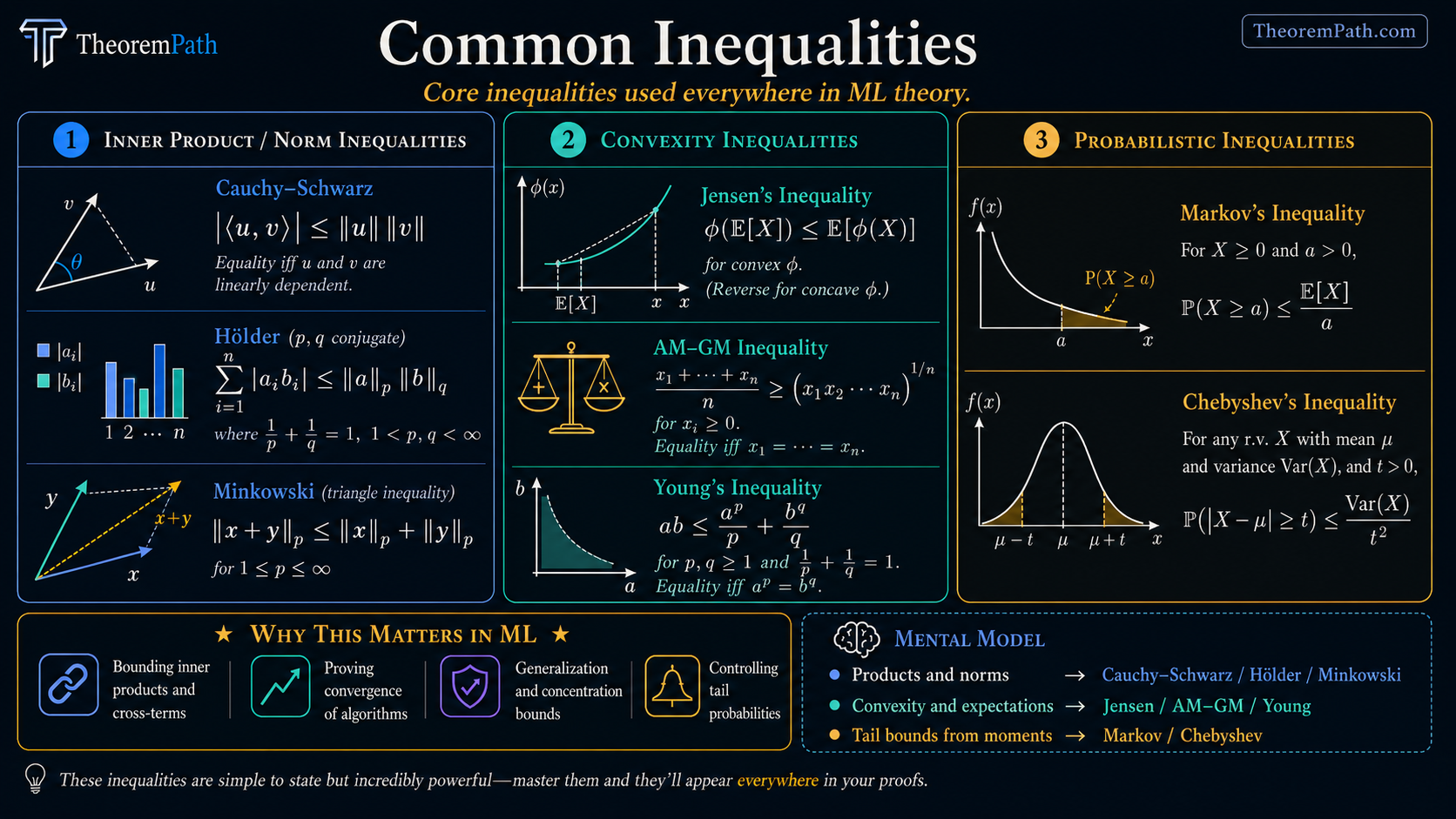
The algebraic and probabilistic inequalities that appear everywhere in ML theory: Cauchy-Schwarz, Jensen, AM-GM, Holder, Minkowski, Young, Markov, and Chebyshev.
Why This Matters
Inequalities are the grammar of mathematical proofs. In ML theory, you cannot write a single generalization bound, convergence proof, or complexity argument without reaching for at least one inequality from this page. Cauchy-Schwarz bounds inner products. Jensen connects to expectations. Markov and Chebyshev give tail bounds.
Two notations recur: for expectation and as the verb of every line.
Hide overviewShow overview
These are not abstract exercises. They are tools you will use on every page of this site. Know them so well that applying them is automatic.
Mental Model
The inequalities on this page fall into three groups:
-
Inner product / norm inequalities: Cauchy-Schwarz, Holder, Minkowski. These relate different norms and inner products. Used to bound terms that involve products or sums.
-
Convexity inequalities: Jensen, AM-GM, Young. These exploit the curvature of convex (or concave) functions. Jensen is the most important single inequality in ML theory.
-
Probabilistic inequalities: Markov, Chebyshev. These bound tail probabilities using moment information. They are the foundation for all concentration inequalities.
Inner Product and Norm Inequalities
Cauchy-Schwarz Inequality
Statement
For any vectors in an inner product space:
Exact statement
LaTeX source for copy/export
|\langle u, v \rangle| \leq \|u\|\,\|v\|Intuition
The inner product of two vectors cannot exceed the product of their lengths. This is a generalization of the fact that .
Proof Sketch
For any , . Expanding:
This is a non-negative quadratic in , so its discriminant is non-positive:
which gives .
Why It Matters
Cauchy-Schwarz is the most frequently used inequality in all of mathematics. In ML theory, it appears when: bounding inner products in kernel methods, analyzing gradient descent geometry, studying Rademacher complexity, and controlling cross-terms in bias-variance decompositions.
Failure Mode
Cauchy-Schwarz gives the tightest possible bound for inner products in terms of norms, but it can still be loose if and are nearly orthogonal (the bound gives while the true value is near zero). When you have structural information about the angle between and , tighter bounds are possible.
Common equivalent forms include:
- Equality case: equality occurs when the two vectors are linearly dependent.
- For random variables: when the second moments exist.
- For finite sums: .
Holder Inequality
For with (conjugate exponents):
Or in integral form: .
Special case: gives Cauchy-Schwarz.
When it arises: Bounding mixed-norm expressions, dual norm computations (), and proving interpolation inequalities. The duality between and norms underpins convex analysis.
Minkowski Inequality (Triangle Inequality for L^p)
For :
In short: .
This is the triangle inequality for norms, proven using Holder. It confirms that is a valid norm for . (For , the triangle inequality fails and is not a norm.)
Convexity Inequalities
Jensen Inequality
Statement
If is a convex function and is a random variable:
If is concave, the inequality reverses: .
Finite form: For weights with :
Exact statement
LaTeX source for copy/export
f(\mathbb{E}[X]) \leq \mathbb{E}[f(X)]Intuition
A convex function "bows upward." The value of at the average point is at most the average of at the individual points. Geometrically: the chord connecting two points on a convex curve lies above the curve.
Proof Sketch
The cleanest sketch uses a subgradient. If is a proper convex function and lies in the relative interior of the domain of , then admits a subgradient at , i.e. for all . Taking expectations:
For convex on , a subgradient (left/right derivative) always exists at interior points, so this argument covers the standard real-valued case. For boundary points, infinite-dimensional settings, or extended-real-valued , one typically falls back on the finite convex-combination version with , (provable by induction on the number of points), and then extends to expectations by an approximation/measure-theoretic argument.
Why It Matters
Jensen is arguably the single most important inequality in ML theory. Applications include:
- EM algorithm: The ELBO is a lower bound on log-likelihood because is concave: .
- KL divergence is non-negative: follows from Jensen applied to .
- Convex loss functions: relates the risk of the average model to the average risk.
- Information theory: entropy bounds, data processing inequality.
Failure Mode
Jensen gives a direction of inequality but not its magnitude. The gap can be anywhere from zero (when is constant or is linear) to very large (when has high variance and is strongly convex). Tighter bounds require knowledge of the variance of and the curvature of .
AM-GM Inequality (Arithmetic Mean - Geometric Mean)
For non-negative reals :
Equality holds if and only if all are equal.
Two-variable form: , or equivalently .
Proof from Jensen: Apply Jensen to the concave function : .
When it arises: Bounding products by sums (which are easier to handle), optimizing expressions involving products, proving convergence rates.
Young Inequality
For and conjugate exponents with :
Special case (): , which is AM-GM for squares.
Parametric form: For any : . This is extremely useful in proofs where you need to "split" a product into two terms with different scaling.
When it arises: Splitting cross-terms in energy estimates, proving Holder from Young, absorbing error terms in convergence proofs. The parametric form lets you trade off how much of the bound goes into each term.
Probabilistic Inequalities
Markov Inequality
If , then for any :
Proof: .
When it arises: Markov is the foundation of all tail bounds. Chebyshev applies Markov to . The Chernoff method applies Markov to . Every concentration inequality starts with Markov.
Limitation: The bound decays as , far too slowly for most applications. You almost always want Hoeffding or Bernstein instead.
Chebyshev Inequality
For any random variable with mean and finite variance :
Proof: Apply Markov to : .
When it arises: Proving weak laws of large numbers, giving initial sample complexity bounds ( to estimate a mean within at confidence ). The polynomial tail is worse than the exponential tails from Hoeffding, but Chebyshev requires only finite variance, not boundedness.
Applications in ML Theory
Here is how each inequality appears in practice:
| Inequality | Typical ML Use |
|---|---|
| Cauchy-Schwarz | Bounding inner products in kernel methods, RKHS norms |
| Holder | Dual norm computations, mixed-norm regularization |
| Jensen ( concave) | EM algorithm ELBO, KL divergence non-negativity |
| Jensen (convex loss) | Relating ensemble risk to average individual risk |
| AM-GM | Bounding products in convergence rate proofs |
| Young (parametric) | Splitting cross-terms with tunable |
| Markov | Starting point for all exponential tail bounds |
| Chebyshev | Quick variance-based concentration when boundedness is unavailable |
Canonical Examples
Jensen in the EM algorithm
The EM algorithm maximizes a lower bound on the log-likelihood. For any distribution over latent variables:
The inequality is Jensen applied to the concave function : . The right-hand side is the ELBO (Evidence Lower BOund).
Cauchy-Schwarz in bounding gradient norms
In gradient descent analysis, you often need to bound . By Cauchy-Schwarz:
This converts an inner product (hard to control) into a product of norms (each of which can be bounded separately).
Young inequality to split cross-terms
In proving convergence of gradient descent, terms like arise (where is an error). Using the parametric Young inequality:
By choosing appropriately, the gradient term can be absorbed into the main descent lemma while the error term is controlled separately.
Common Confusions
Jensen goes the wrong way for concave functions
For convex : . For concave : .
Students frequently apply Jensen to (concave) and get the direction wrong. Remember: (concave Jensen), which gives and the EM lower bound.
Cauchy-Schwarz is a special case of Holder, not the other way around
Holder with gives Cauchy-Schwarz. Holder is strictly more general (it works for any conjugate pair ). But Cauchy-Schwarz is by far the most commonly used special case.
Summary
- Cauchy-Schwarz: . the universal inner product bound
- Holder: . generalizes CS to spaces
- Jensen: for convex . The most important inequality in ML theory
- AM-GM: arithmetic mean geometric mean. bounds products by sums
- Young: . splits products with tunable balance
- Markov: . foundation of all tail bounds
- Chebyshev: . variance-based tails
Exercises
Problem
Assume (i.e., wherever , so is -a.s. finite). Use Jensen's inequality to show that the KL divergence is non-negative: . What happens to if is not absolutely continuous with respect to ?
Problem
Use the parametric Young inequality to prove that for any and : .
Problem
Prove Holder's inequality for sums: if with , then .
References
Canonical:
- Axler, Linear Algebra Done Right (2024), Chapter 6 for inner-product spaces
- Hardy, Littlewood, Polya, Inequalities (1934). The classic reference
- Steele, The Cauchy-Schwarz Master Class (2004). excellent problem-driven treatment
Current:
- Boucheron, Lugosi, Massart, Concentration Inequalities (2013), Chapter 1
- Cover & Thomas, Elements of Information Theory (2006), Chapter 2 for Jensen applications
Next Topics
Building on these foundational inequalities:
- Concentration inequalities: exponential tail bounds that build on Markov and Chebyshev
- Convex optimization basics: where convexity inequalities become algorithmic
- Empirical risk minimization: where everything comes together
Last reviewed: April 26, 2026
Canonical graph
Required before and derived from this topic
These links come from prerequisite edges in the curriculum graph. Editorial suggestions are shown here only when the target page also cites this page as a prerequisite.
Required prerequisites
2- Common Probability Distributionslayer 0A · tier 1
- Kolmogorov Probability Axiomslayer 0A · tier 1
Derived topics
4- Concentration Inequalitieslayer 1 · tier 1
- Convex Optimization Basicslayer 1 · tier 1
- Empirical Risk Minimizationlayer 2 · tier 1
- Convex Tinkeringlayer 2 · tier 2
Graph-backed continuations