Fokker–Planck Equation

Why This Matters

Solving an SDE gives you sample paths; solving its Fokker–Planck equation gives you the density of those paths at every time. For most ML applications you do not actually want one trajectory. You want to know what distribution your sampler is converging to, how fast it gets there, and whether any of that depends on a hyperparameter you can tune. Those are PDE questions, not SDE questions, and the Fokker–Planck equation is what turns one into the other.

Hide overviewShow overview

This is why the Fokker–Planck equation shows up implicitly under nearly every sampling and generative-modeling result in modern ML. The stationary density of Langevin dynamics is the kernel of its Fokker–Planck operator; the convergence rate of SGLD and ULA is the spectral gap of that operator; the forward noising process in diffusion models is a Fokker–Planck PDE evolving the data distribution toward standard Gaussian; the score-matching loss is a re-expression of one term in the Fokker–Planck operator.

The same equation also appears in physics (chemical kinetics, polymer dynamics, plasma transport), finance (option pricing under nonconstant volatility), and biology (population genetics under drift). It is one of the densest cross-disciplinary PDEs you can learn.

Mental Model

An SDE pushes a single particle around with drift $b$ and noise $\sigma$. If you instead release a cloud of independent particles all from the same initial distribution and watch their density $p(x, t)$ evolve, that density satisfies a deterministic PDE: the drift $b$ advects the cloud, and the noise $\sigma$ smears it. The Fokker–Planck equation is exactly this advection–diffusion PDE. The smearing is anisotropic and position-dependent because $\sigma$ can be a matrix that varies with $x$.

A useful aphorism: the SDE is the Lagrangian view (follow one particle), the Fokker–Planck equation is the Eulerian view (watch the field of particles). They contain the same information, expressed in dual languages.

Formal Derivation

Definition

Fokker–Planck Equation (Forward Kolmogorov)${\partial }_{t}p=-\nabla \cdot (bp)+\frac{1}{2}{\sum }_{i,j}{\partial }_i{\partial }_j\left((\sigma {\sigma }^{\top }{)}_{ij}p\right)$

Let $X_t \in \mathbb{R}^d$ solve the Itô SDE $dX_t = b(X_t, t)\,dt + \sigma(X_t, t)\,dB_t$ with $X_0 \sim p_0$, and suppose $X_t$ admits a smooth density $p(x, t)$. Then $p$ satisfies

$$\partial_t p(x, t) = -\sum_{i=1}^d \partial_i \big(b_i(x, t)\, p(x, t)\big) + \tfrac{1}{2} \sum_{i,j=1}^d \partial_i \partial_j \big( D_{ij}(x, t)\, p(x, t) \big),$$

with diffusion tensor $D = \sigma \sigma^\top$, initial condition $p(x, 0) = p_0(x)$, and decay-at-infinity boundary conditions.

The right-hand side is the forward Kolmogorov operator $\mathcal{L}^* p$. Its formal adjoint $\mathcal{L} f = b \cdot \nabla f + \tfrac{1}{2} \operatorname{Tr}(D \nabla^2 f)$ is the infinitesimal generator of the SDE.

Theorem

Fokker–Planck Derivation from Itô

Statement

Under the assumptions above, for every test function $f \in C_c^\infty(\mathbb{R}^d)$ and time $t \ge 0$, $\frac{d}{dt} \mathbb{E}[f(X_t)] = \mathbb{E}[\mathcal{L} f(X_t)]$. Writing this as $\int f\, \partial_t p\,dx = \int (\mathcal{L} f)\, p\,dx$ and integrating by parts gives $\partial_t p = \mathcal{L}^* p$ as a distributional identity, which equals the Fokker–Planck equation in the display above.

Intuition

The generator $\mathcal{L}$ is "what happens to the expectation of a function as the particle moves." Its adjoint flips the perspective: "what happens to the density as the cloud of particles moves." The Itô formula gives the first; integration by parts trades it for the second.

Proof Sketch

By Itô, $df(X_t) = \mathcal{L} f(X_t)\,dt + (\nabla f)^\top \sigma\,dB_t$. The stochastic integral is a martingale (test functions have compact support), so $\mathbb{E}[f(X_t)] = \mathbb{E}[f(X_0)] + \int_0^t \mathbb{E}[\mathcal{L} f(X_s)]\,ds$. Differentiating in $t$ and writing both sides as integrals against $p(\cdot, s)$ gives $\int f\, \partial_s p = \int (\mathcal{L} f)\, p = \int f\, (\mathcal{L}^* p)$ for every $f$, which forces $\partial_s p = \mathcal{L}^* p$ pointwise on the support.

Why It Matters

Every claim about "what distribution the SDE converges to" or "how fast it mixes" is, formally, a claim about $\mathcal{L}^*$. Spectral analysis of $\mathcal{L}^*$ gives mixing rates; null-space analysis gives stationary distributions; positivity and mass-conservation properties live in the PDE. None of this is visible from the SDE itself. The density $p$ satisfies $\partial_t p = -\nabla \cdot (bp) + \tfrac{1}{2} \sum_{i,j} \partial_i \partial_j ((\sigma\sigma^\top)_{ij}\, p)$ in the weak sense.

Failure Mode

The derivation assumes a smooth density exists. SDEs with degenerate or state-dependent diffusion (e.g., CIR near zero, hypoelliptic systems where $\sigma$ is rank-deficient) may have singular or measure-valued solutions to the Fokker–Planck equation, requiring the framework of Hörmander's theorem or Malliavin calculus. The clean PDE form is restricted to elliptic / uniformly nondegenerate diffusions.

report a correction →

Stationary Distributions

A stationary density $p_\infty$ is a fixed point of the Fokker–Planck flow: $\mathcal{L}^* p_\infty = 0$. For the canonical "overdamped Langevin" SDE $dX_t = -\nabla U(X_t)\,dt + \sqrt{2/\beta}\,dB_t$ with potential $U$ and inverse temperature $\beta$, the stationary distribution is the Gibbs measure

$$p_\infty(x) = \frac{1}{Z} e^{-\beta U(x)}, \qquad Z = \int e^{-\beta U(x)}\,dx.$$

Plug it into $\mathcal{L}^*$ and the drift and diffusion terms cancel exactly. This is the entire foundation of MCMC sampling from energy-based models, of SGLD as approximate Bayesian inference, and of the equilibrium statistical mechanics that generative models implicitly target.

For non-reversible SDEs (those with drift not equal to $-\nabla U$ for any $U$), the stationary distribution still exists when $\mathcal{L}^*$ has a one-dimensional kernel, but it is no longer Gibbs and the analysis is much harder.

Convergence Rates and Spectral Gap

The Fokker–Planck operator on $L^2(p_\infty)$ is self-adjoint and negative semidefinite for reversible (Langevin) dynamics, with $0$ as a simple eigenvalue and eigenvector $p_\infty$. The next eigenvalue $-\lambda_1 < 0$ controls exponential convergence:

$$\lVert p(\cdot, t) - p_\infty \rVert_{L^2(1/p_\infty)}^2 \le e^{-2 \lambda_1 t}\, \lVert p_0 - p_\infty \rVert_{L^2(1/p_\infty)}^2.$$

The constant $\lambda_1$ is the spectral gap, and Bakry–Émery theory gives sharp lower bounds in terms of the convexity of $U$: for the overdamped Langevin SDE $dX_t = -\nabla U(X_t)\,dt + \sqrt{2/\beta}\,dB_t$, if $\nabla^2 U \succeq m\, I$ for some $m > 0$, then $\lambda_1 \ge m$ and the law of $X_t$ converges exponentially fast at rate $m$. The temperature $\beta$ cancels: warmer noise (larger $\beta^{-1}$) accelerates diffusion but the effective potential entering the stationary measure is $\beta U$, which has convexity $\beta m$, and these two effects exactly compensate. The OU process $dX = -\theta X\,dt + \sigma\,dB_t$ is the canonical sanity check: $U(x) = \tfrac{1}{2}\theta x^2$ gives $m = \theta$, and the Bakry–Émery bound predicts $\lambda_1 \ge \theta$, which matches the exact spectrum below regardless of $\sigma$. This is the cleanest statement of "Langevin mixes fast on log-concave targets," and it is the theoretical underpinning of every convergence guarantee for gradient-based MCMC on convex problems.

The stronger log-Sobolev inequality

$$\operatorname{Ent}_{p_\infty}(f^2) \le \frac{2}{\rho_{\text{LSI}}} \mathbb{E}_{p_\infty}[\lVert \nabla f \rVert^2]$$

implies the same exponential rate in KL divergence, not just $L^2$, and is the right tool whenever you need entropic — not energetic — convergence guarantees.

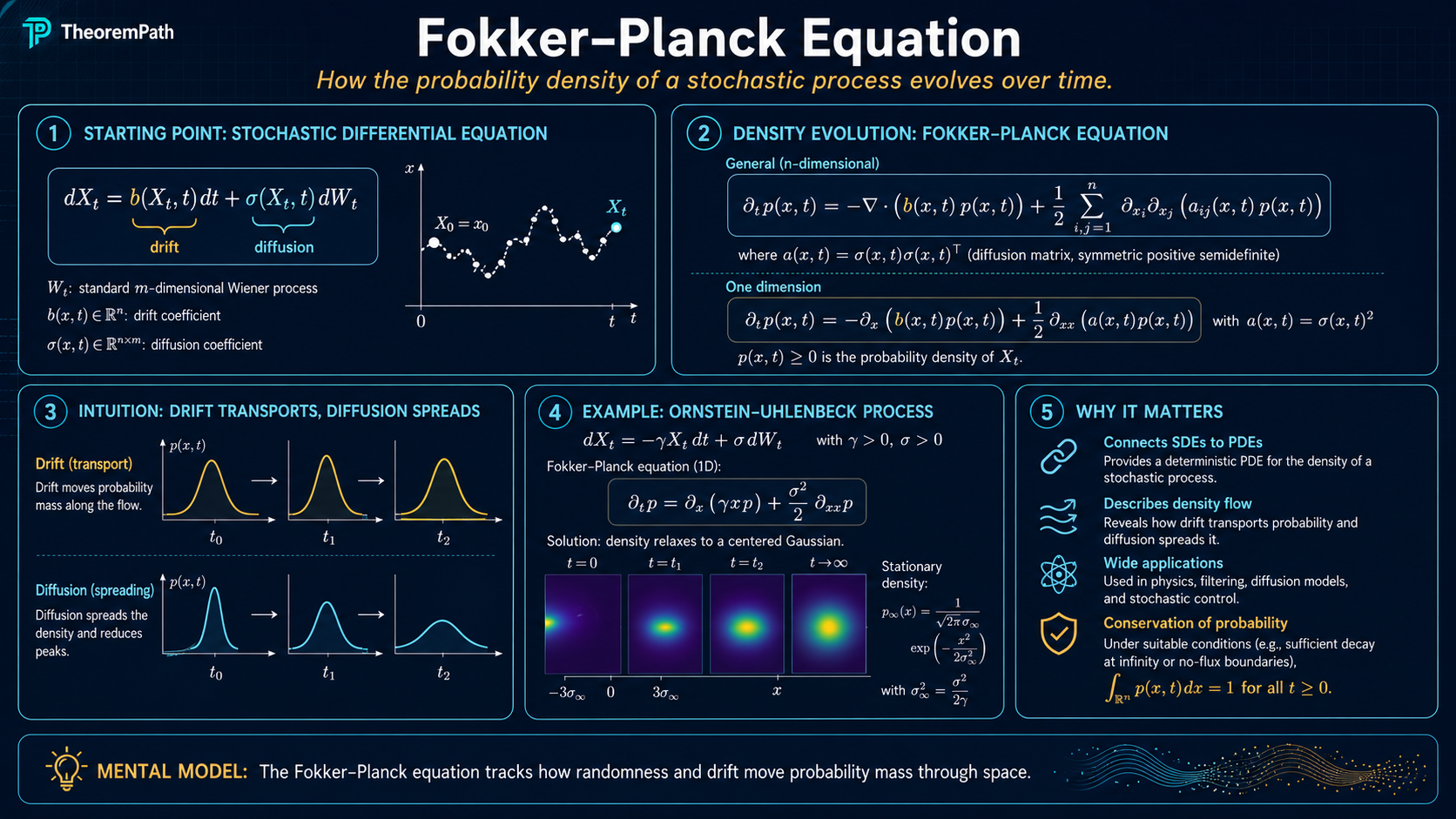
Worked Example: Ornstein–Uhlenbeck Density

Take $dX_t = -\theta X_t\,dt + \sigma\,dB_t$ in $\mathbb{R}$. The Fokker–Planck equation is $\partial_t p = \theta \partial_x (x\, p) + \tfrac{1}{2} \sigma^2 \partial_{xx} p$. With Gaussian initial data $X_0 \sim \mathcal{N}(\mu_0, v_0)$ the solution stays Gaussian with

$$\mu(t) = e^{-\theta t} \mu_0, \qquad v(t) = e^{-2\theta t} v_0 + \frac{\sigma^2}{2\theta}\big(1 - e^{-2\theta t}\big).$$

The stationary distribution is $\mathcal{N}(0, \sigma^2/(2\theta))$, exactly the Gibbs measure $e^{-\beta U}/Z$ for $U(x) = \tfrac{1}{2}\theta x^2$ and $\beta = 2 \theta / \sigma^2$. The spectral gap is $\theta$ — the same $\theta$ that controls mean-reversion in the SDE, so the SDE and PDE views agree on the convergence rate, as they must.

Common Confusions

Watch Out

Forward Kolmogorov vs backward Kolmogorov are different equations

The Fokker–Planck equation is the forward Kolmogorov equation: it evolves the density of $X_t$ forward in time. The backward Kolmogorov equation $\partial_t u + \mathcal{L} u = 0$ with terminal condition $u(T, x) = g(x)$ evolves the value function $u(t, x) = \mathbb{E}[g(X_T) \mid X_t = x]$ backward in time and uses the generator $\mathcal{L}$, not its adjoint. Forward asks "where will the particle be?", backward asks "what is the expected payoff if it ends here?". The Feynman–Kac formula and the deep BSDE method live in the backward picture.

Watch Out

The diffusion tensor is σσ^⊤, not σ

A common bug is to write the second derivative term as $\partial_i \partial_j (\sigma_{ij} p)$ instead of $\partial_i \partial_j ((\sigma \sigma^\top)_{ij} p)$. The diffusion enters the Fokker–Planck equation only through its covariance matrix $D = \sigma \sigma^\top$; two SDEs with the same drift and the same $\sigma \sigma^\top$ have the same Fokker–Planck equation, even if their $\sigma$ matrices differ (e.g., differ by a right rotation). This is also why diffusion models can use scalar noise schedules without losing generality.

Watch Out

A stationary distribution is not the same as a steady-state flux

$\mathcal{L}^* p = 0$ has two meaningful sub-cases. Reversible (Langevin) dynamics: drift $b = -\nabla U$ and the equilibrium current $J = b p_\infty - \tfrac{1}{2} D \nabla p_\infty$ is identically zero — the system is in detailed balance. Non-reversible dynamics: $\mathcal{L}^* p_\infty = 0$ but $J \ne 0$; the system has steady probability currents, only their divergence vanishes. Non-reversible Langevin samplers exploit exactly this to mix faster than reversible ones; they sit at a stationary distribution but with persistent rotational flow.

Exercises

ExerciseCore

Problem

Verify by direct substitution that the Gibbs measure $p_\infty(x) = e^{-\beta U(x)}/Z$ is stationary for the overdamped Langevin SDE $dX_t = -\nabla U(X_t)\,dt + \sqrt{2/\beta}\,dB_t$. Identify the cancellation that makes this work.

Hint

Reveal Solution

ExerciseAdvanced

Problem

For the OU process $dX_t = -\theta X_t\,dt + \sigma\,dB_t$, compute the full spectrum of the Fokker–Planck operator on $L^2(p_\infty)$. Show that the eigenvalues are $-n \theta$ for $n = 0, 1, 2, \dots$ and identify the corresponding eigenfunctions.

Hint

Reveal Solution

References

Canonical:

• Risken, The Fokker–Planck Equation: Methods of Solution and Applications (2nd ed., Springer, 1989). The standard physics-flavored reference; Chapters 4-6 cover the canonical-form derivation, stationary solutions, and eigenfunction expansions.
• Karatzas and Shreve, Brownian Motion and Stochastic Calculus (2nd ed., Springer, 1991), Chapter 5.7. SDE-side derivation of the forward and backward Kolmogorov equations.
• Stroock and Varadhan, Multidimensional Diffusion Processes (Springer, 1979). Rigorous treatment of the martingale-problem formulation, useful when coefficients are non-smooth.
• Pavliotis, Stochastic Processes and Applications (Springer, 2014). Chapters 4 and 5 give the cleanest modern treatment, with explicit Bakry-Emery / log-Sobolev material in Chapter 6.

Current:

• Bakry, Gentil, and Ledoux, Analysis and Geometry of Markov Diffusion Operators (Springer Grundlehren, 2014). The authoritative reference on functional inequalities for diffusion semigroups; Chapters 4-6 give the curvature-dimension framework that yields exponential convergence.
• Villani, Optimal Transport: Old and New (Springer, 2009), Chapters 21-25. The Otto-calculus / gradient-flow viewpoint: Fokker-Planck as the Wasserstein gradient flow of relative entropy.
• Markowich and Villani, On the Trend to Equilibrium for the Fokker-Planck Equation: An Interplay Between Physics and Functional Analysis (Matematica Contemporanea 19, 2000). The reference paper on entropy methods for convergence rates.

Next Topics

• Langevin Dynamics: the canonical SDE whose Fokker–Planck equation has a Gibbs stationary distribution.
• Score Matching: training a network on the score $\nabla \log p$ that appears inside the Fokker–Planck operator.
• Diffusion Models: forward noising SDEs and their Fokker–Planck duals; reverse-time samplers.
• Time Reversal of SDEs: how the reversed SDE's drift involves the score $\nabla \log p$ that the forward Fokker–Planck operator already contains.
• SGD as SDE: SGD viewed as a discretization of a Langevin-type SDE; the implicit Fokker–Planck equation for SGD's stationary distribution.