Mathematical Infrastructure
Ito's Lemma
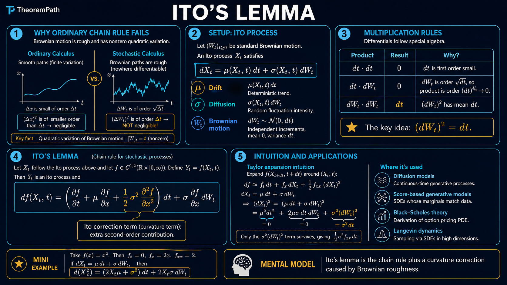
The chain rule of stochastic calculus: if a process follows an SDE, applying a smooth function to it yields a modified SDE with an extra second-order correction term that has no analogue in ordinary calculus.
Prerequisites
Why This Matters
In ordinary calculus, if you know and want , you apply the chain rule: . In stochastic calculus, this formula is wrong. The chain rule picks up an extra term proportional to . This correction term is the reason stochastic calculus exists as a separate subject.
Hide overviewShow overview
Every derivation in diffusion models, score-based generative models, and mathematical finance uses Ito's lemma. If you cannot apply it mechanically, you cannot read these papers.
Ito Isometry
Before stating the chain rule, we record the core identity that makes the Ito integral well-defined as an object.
Ito Isometry
Statement
For adapted to the filtration of :
Intuition
The stochastic integral is a linear isometry from the Hilbert space of adapted square-integrable processes (with the inner product) into . Variance on the left equals expected energy on the right.
Why It Matters
This identity is how the Ito integral is constructed. Simple processes satisfy it by direct computation. General adapted processes are defined as limits of simple processes, and the isometry guarantees the limit exists and is unique. Every existence and uniqueness proof for SDEs rests on it.
Mental Model
A Brownian motion path is so rough that does not vanish. It equals in a precise sense (quadratic variation). When you Taylor expand , the second-order term survives because contains a piece. In ordinary calculus, . In stochastic calculus, .
Setup
Let be an Ito process satisfying the SDE:
where is standard Brownian motion, is the drift, and is the diffusion coefficient.
Quadratic Variation Rule
The multiplication rules for Ito calculus are:
These rules follow from the quadratic variation of Brownian motion: .
Main Theorems
Ito's Lemma (One Dimension)
Statement
Let . Then satisfies:
The term is the Ito correction. It has no analogue in ordinary calculus.
Intuition
Taylor expand to second order. The first-order terms give the ordinary chain rule. The second-order term normally vanishes, but here . So survives.
Proof Sketch
Partition into subintervals. Write the telescoping sum . Taylor expand each increment to second order. The first-order terms converge to the Ito integral. The second-order terms converge to because of the quadratic variation of . Cross terms and higher-order terms vanish in .
Why It Matters
This is the computational workhorse of stochastic calculus. Every application requires you to start with a process and compute the dynamics of some function of it. Without Ito's lemma, you cannot derive the Black-Scholes equation, compute the SDE for the score function in diffusion models, or analyze Langevin dynamics.
Failure Mode
The formula requires . If is not twice differentiable (e.g., ), the standard Ito lemma does not apply. You need the Tanaka-Meyer formula, which introduces local time. Also, this is the Ito version. The Stratonovich chain rule has no correction term but changes the integral definition.
Canonical Examples
Geometric Brownian Motion
Let satisfy (stock price model). Apply Ito's lemma to . We have and .
So is a Brownian motion with drift . The correction term is why the expected log return is less than .
Square of Brownian motion
Let . Here , , , .
Integrating: . This gives the Ito integral identity .
Multidimensional Ito's Lemma
Statement
If , then for :
where .
Intuition
The same idea as the 1D case, but now the quadratic covariation between different components contributes through the full Hessian matrix of .
Proof Sketch
Same Taylor expansion argument as the 1D case, applied componentwise. The cross terms contribute through the covariation .
Why It Matters
Diffusion models in high dimensions (image generation) operate on multidimensional SDEs. The multivariate version is needed to derive the reverse-time SDE and the score matching objective.
Failure Mode
Same regularity requirements as the 1D case, but now applied to all partial derivatives up to second order.
Common Confusions
Why not just use the ordinary chain rule?
Because . Brownian paths have infinite total variation on any interval, so the second-order term in the Taylor expansion does not vanish. If you apply the ordinary chain rule, you get the wrong drift. The geometric Brownian motion example shows this: the ordinary chain rule gives drift for , but the correct drift is .
Ito vs Stratonovich
In Stratonovich calculus, the chain rule has no correction term: . The price is that the Stratonovich integral is defined as a midpoint Riemann sum, not an endpoint sum. Ito integrals are martingales (useful for probability arguments). Stratonovich integrals obey the ordinary chain rule (useful for physics). They are related by: the Ito SDE corresponds to the Stratonovich SDE .
Feynman-Kac Formula
Ito's lemma gives a direct bridge between parabolic PDEs and SDEs. For a PDE of the form with terminal condition , the solution has the probabilistic representation where follows . The derivation is one line of Ito: apply the lemma to and the PDE kills the drift, leaving a martingale whose expectation reduces to the terminal value. This identity is the foundation of Black-Scholes pricing and also underlies the reverse-time SDE construction in score-based generative models.
Summary
- The Ito correction term is
- It exists because , not zero
- For of geometric Brownian motion, the correction gives drift
- The Ito integral , not as the ordinary chain rule would give
Exercises
Problem
Apply Ito's lemma to . What SDE does satisfy?
Problem
Let satisfy (Ornstein-Uhlenbeck process). Apply Ito's lemma to and use it to compute given .
References
Canonical:
- Oksendal, B. (2003). Stochastic Differential Equations, 6th ed. Springer. Chapters 3-4 (Ito integral, Ito's formula).
- Karatzas, I. and Shreve, S. (1991). Brownian Motion and Stochastic Calculus, 2nd ed. Springer. Chapter 3 (stochastic integration).
- Shreve, S. (2004). Stochastic Calculus for Finance II. Springer. Chapter 4.
- Le Gall, J.-F. (2016). Brownian Motion, Martingales, and Stochastic Calculus. Springer. Chapter 5.
Current:
- Song et al., "Score-Based Generative Modeling through SDEs" (2021), Appendix A.
Next Topics
- Diffusion models: the primary ML application of Ito's lemma today
- Flow matching: an alternative to diffusion that avoids SDEs but relates to them
Last reviewed: April 18, 2026
Canonical graph
Required before and derived from this topic
These links come from prerequisite edges in the curriculum graph. Editorial suggestions are shown here only when the target page also cites this page as a prerequisite.
Required prerequisites
1- Stochastic Calculus for MLlayer 3 · tier 3
Derived topics
5- Diffusion Modelslayer 4 · tier 1
- Backward Stochastic Differential Equationslayer 3 · tier 2
- Feynman–Kac Formulalayer 3 · tier 2
- Stochastic Differential Equationslayer 3 · tier 2
- Flow Matchinglayer 4 · tier 2