Concentration Probability
Measure Concentration and Geometric Functional Analysis
High-dimensional geometry is counterintuitive: Lipschitz functions concentrate, random projections preserve distances, and most of a sphere's measure sits near the equator. Johnson-Lindenstrauss, Gaussian concentration, and Levy's lemma.
Why This Matters
High-dimensional spaces behave nothing like low-dimensional ones. In with , a random vector is almost surely close to in norm. Two independent random unit vectors are almost surely nearly orthogonal. A Lipschitz function of a Gaussian vector is almost surely close to its mean.
Hide overviewShow overview
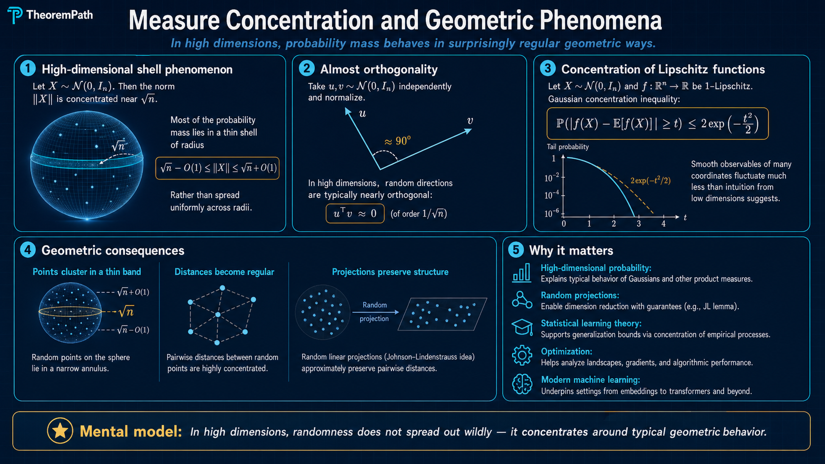
These phenomena are not curiosities. They are the reason dimensionality reduction works, random projections preserve structure, and empirical averages concentrate. The Johnson-Lindenstrauss lemma, which enables practical dimensionality reduction from to , is a direct consequence of Gaussian concentration.
concentration geometry
High dimension turns randomness into a narrow geometric ledger
The proofs below keep repeating the same move: prove one random quantity is close to its mean, then pay a union-bound price to make the statement uniform over many objects.
Thin shell
The coordinates are random, but the normalized radius becomes predictable in high dimension.
Equator belt
most area is near any equatorA random point on a large sphere has tiny projection onto any fixed direction.
Distance ledger
distances stay withinA random projection concentrates every pairwise distance once k is large enough.
one variable
Gaussian concentration controls one Lipschitz observation of a random vector.
many pairs
Johnson-Lindenstrauss repeats that bound over all point pairs.
sphere
Levy concentration says most surface area is trapped near level sets.
The Visual Spine
The page has three objects to keep straight:
- A Gaussian vector has many random coordinates, but its radius is almost deterministic after normalization by .
- A high-dimensional sphere puts most surface area near any equator, so a fixed coordinate or projection is usually small.
- A random projection preserves a finite cloud because every pairwise distance concentrates, and the union bound only costs .
Use the High-Dimensional Probability Lab alongside this page. The lab shows the thin-shell picture, random matrix spectra, and spiked PCA thresholds; this page gives the theorem statements and proof templates behind those pictures.
Gaussian Concentration
Lipschitz Function
A function is -Lipschitz if and only if
for all . The smallest such is the Lipschitz constant.
Gaussian Concentration of Lipschitz Functions
Statement
Let and be -Lipschitz. Then for all :
The function is sub-Gaussian with parameter .
Intuition
Each coordinate of contributes independently to , and the Lipschitz condition limits how much each coordinate can influence the output. The independent contributions each have bounded effect, and their sum concentrates by the same mechanism as a sum of bounded random variables. The dimension does not appear in the bound.
Proof Sketch
Use the Gaussian Poincare inequality:
For the tail bound, apply the Herbst argument: compute the log-MGF
show using the Gaussian log-Sobolev inequality, and then apply the Chernoff bound.
Why It Matters
This single result has enormous consequences. It implies that the norm concentrates around , inner products concentrate around 0, and random projections preserve distances. Most of high-dimensional probability follows from applying this inequality to appropriately chosen Lipschitz functions.
Failure Mode
The result requires Gaussianity (or more generally, a distribution satisfying a log-Sobolev inequality). For heavy-tailed distributions, Lipschitz functions do not concentrate at the Gaussian rate. The bound also requires to be globally Lipschitz; local Lipschitz conditions are not sufficient.
Johnson-Lindenstrauss Lemma
Johnson-Lindenstrauss Lemma
Statement
For any set of points and any , there exists a linear map with
such that for all pairs ,
The map where is a matrix with i.i.d. entries works with high probability.
Intuition
A random projection of a vector has squared norm that concentrates around . This is because
The sum of squared Gaussians concentrates around its mean by chi-squared concentration. Taking a union bound over all pairs gives the result.
Proof Sketch
Fix a single pair and let . Then
i.i.d. By sub-exponential concentration of chi-squared random variables,
For , choosing and applying a union bound over pairs gives failure probability at most , which is small for large enough.
Why It Matters
This lemma says that points in arbitrarily high dimension can be embedded into dimensions while approximately preserving all pairwise distances. The target dimension depends only on and , not on the original dimension . This is the theoretical foundation for random projection methods in dimensionality reduction, approximate nearest neighbor search, and compressed sensing.
Failure Mode
The target dimension is tight: there exist point sets requiring dimensions for any linear map. For very small, the target dimension can still be large. The lemma also only preserves Euclidean distances; other metrics require different techniques.
From one vector to all pairs
Gaussian concentration usually starts with one random quantity. For JL, the one-pair statement is:
There are fewer than pairs. A union bound therefore asks for
Solving this inequality gives . The dimension reduction theorem is not magic: it is one chi-squared tail bound plus a union bound over pairs.
Concentration on the Sphere
Levy's Lemma (Concentration on the Sphere)
Statement
Let be uniformly distributed on and be -Lipschitz. Let be the median of . Then:
The concentration improves with dimension: higher dimension means tighter concentration.
Intuition
On a high-dimensional sphere, most of the surface area is concentrated near any equator. A Lipschitz function cannot vary much on this concentrated strip. The effective number of "independent directions" on the sphere is , which is why the exponent contains .
Proof Sketch
The proof uses the spherical isoperimetric inequality: among all sets of a given measure on , spherical caps have the smallest boundary. For a cap of measure (the hemisphere), the -enlargement has measure at least
For a Lipschitz function, the set contains the -enlargement of .
Why It Matters
Levy's lemma makes precise the idea that high-dimensional spheres are "effectively one-dimensional" from the perspective of Lipschitz functions. Any continuous measurement on a high-dimensional sphere will give nearly the same value for almost every point. This is a key ingredient in proofs of the Johnson-Lindenstrauss lemma via spherical projections.
Failure Mode
The bound degrades for non-Lipschitz functions. For discontinuous functions or functions with large Lipschitz constant relative to the sphere's radius, the concentration is useless. The bound is also trivial in low ambient dimension: under the convention , the case gives , two points rather than a circle. The circle is , corresponding to . For , the exponent is only
so the bound gives the usual one-dimensional Gaussian tail rate, with no dimensional improvement. The concentration becomes useful once is large.
Why High-Dimensional Geometry is Counterintuitive
Three specific phenomena that defy low-dimensional intuition:
-
Norm concentration: if , then in probability. The norm is approximately deterministic.
-
Near-orthogonality: if independently, then has standard deviation . Random vectors are nearly orthogonal.
-
Volume in corners: most of the volume of a high-dimensional cube is near the corners (near radius ), not near the center. The inscribed ball has negligible volume for large .
Common Confusions
JL says nothing about structure preservation beyond distances
The JL lemma preserves pairwise Euclidean distances. It does not preserve cluster structure, manifold geometry, or topological properties. Two point sets with the same pairwise distance matrix are mapped identically by JL. For structure beyond distances, you need methods like t-SNE or UMAP that optimize different objectives.
Gaussian concentration dimension-free does not mean dimension irrelevant
The bound
does not contain , but the Lipschitz constant and the mean can depend on . For example, is -Lipschitz with mean approximately . The bound says deviates from by at most , which is a relative deviation of .
Summary
- Lipschitz functions of Gaussians are sub-Gaussian with parameter equal to the Lipschitz constant. No dependence on dimension.
- JL: points in can be projected to dimensions, preserving distances up to .
- Levy's lemma: on , concentration improves with dimension
- High-dimensional norm concentrates: for .
- Random vectors are nearly orthogonal in high dimensions
Exercises
Problem
Let . Show that is -Lipschitz and use Gaussian concentration to bound
Problem
Prove the JL lemma for a single pair: if and with having i.i.d. entries, show that
for .
References
Canonical:
- Vershynin, High-Dimensional Probability, Chapters 5 and 8
- Ledoux, The Concentration of Measure Phenomenon (2001)
Current:
-
Boucheron, Lugosi, Massart, Concentration Inequalities, Chapter 5
-
Wainwright, High-Dimensional Statistics (2019), Chapter 2
-
van Handel, Probability in High Dimension (2016), Chapters 1-3
Next Topics
- Matrix concentration: replace scalar deviations with operator-norm deviations
- Empirical processes and chaining: applying concentration to suprema of random functions
- Dimensionality reduction theory: use random projections as an algorithmic primitive
Last reviewed: April 21, 2026
Canonical graph
Required before and derived from this topic
These links come from prerequisite edges in the curriculum graph. Editorial suggestions are shown here only when the target page also cites this page as a prerequisite.
Required prerequisites
2- Sub-Gaussian Random Variableslayer 2 · tier 1
- Epsilon-Nets and Covering Numberslayer 3 · tier 1
Derived topics
3- Matrix Concentrationlayer 3 · tier 1
- Dimensionality Reduction Theorylayer 2 · tier 2
- Empirical Processes and Chaininglayer 3 · tier 2
Graph-backed continuations