Proper Scoring Rules

Why This Matters

When a model outputs a probability (e.g., "70% chance of rain"), you want that probability to mean something. A model that says 70% should be right about 70% of the time. The question is: does the loss function you use to train or evaluate the model incentivize this honest reporting?

Hide overviewShow overview

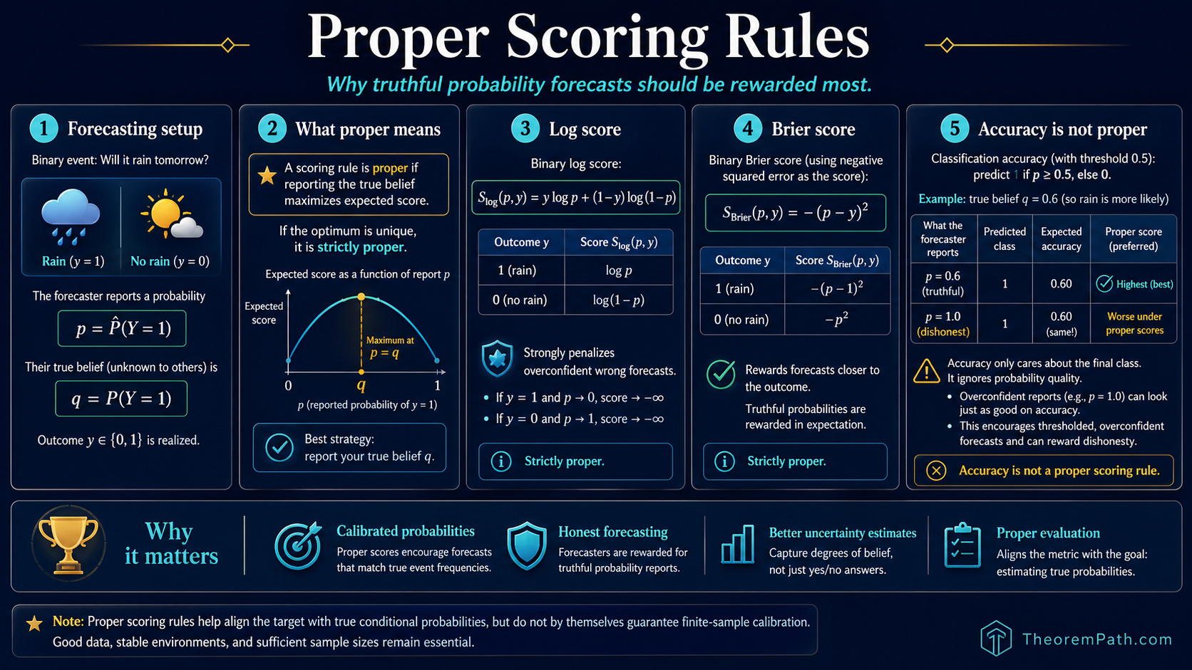
A proper scoring rule says yes: the forecaster's expected score is maximized when they report their true belief. An improper scoring rule can be gamed: the forecaster can get a better expected score by reporting a probability different from their true belief.

Cross-entropy loss (log score) is strictly proper. Brier score (squared error on probabilities) is strictly proper. Classification accuracy is not proper. Properness gives the right target: for a strictly proper rule, the population-optimal forecast is the true conditional probability. It does not automatically deliver a calibrated finite-sample model: a deep network trained with cross-entropy is well known to be miscalibrated in practice (Guo et al. 2017), because optimization, model misspecification, and overfitting all break the population-optimum argument. Training with a proper scoring rule rules out the gross failure modes of training with an improper one (e.g., accuracy), but does not by itself produce calibrated probabilities.

Mental Model

Imagine a weather forecaster who believes there is a 60% chance of rain. A proper scoring rule rewards her most if she reports 60%. If she reports 90% instead (to seem more decisive), her expected score is worse. If she reports 50% (hedging), her expected score is also worse. Only the truth maximizes expected score.

An improper rule might reward her more for reporting 100% or 0% (confident and sometimes right) than for reporting her honest 60%.

Formal Setup

Definition

Scoring Rule$S(p,y)$

A scoring rule assigns a numerical score $S(p, y)$ to a probability forecast $p \in [0,1]$ (or more generally $p \in \Delta_K$ for $K$ classes) given the realized outcome $y$. Higher scores indicate better forecasts (we follow the convention that scoring rules are to be maximized).

Definition

Proper Scoring Rule

A scoring rule $S$ is proper if and only if for all true probabilities $q$ and all reported probabilities $p$:

$\mathbb{E}_{y \sim q}[S(q, y)] \geq \mathbb{E}_{y \sim q}[S(p, y)]$

The forecaster maximizes expected score by reporting $p = q$. The rule is strictly proper if and only if equality holds only when $p = q$.

Main Scoring Rules

Definition

Log Score$S_{\log }$

For binary outcomes with $y \in \{0, 1\}$:

$S_{\log}(p, y) = y \ln p + (1 - y) \ln(1 - p)$

The negative log score is the cross-entropy loss: $-S_{\log}(p, y) = -y \ln p - (1-y) \ln(1-p)$.

Definition

Brier Score$S_{\text{Brier}}$

For binary outcomes:

$S_{\text{Brier}}(p, y) = -(p - y)^2$

This is the negative of the squared difference between the forecast probability and the outcome. Lower squared error means higher Brier score.

Main Theorems

Theorem

Log Score and Brier Score Are Strictly Proper

Statement

The log score $S_{\log}$ and the Brier score $S_{\text{Brier}}$ are both strictly proper. For the log score:

$\mathbb{E}_{y \sim q}[S_{\log}(q, y)] - \mathbb{E}_{y \sim q}[S_{\log}(p, y)] = \text{KL}(q \| p) \geq 0$

with equality iff $p = q$. For the Brier score:

$\mathbb{E}_{y \sim q}[S_{\text{Brier}}(q, y)] - \mathbb{E}_{y \sim q}[S_{\text{Brier}}(p, y)] = (p - q)^2 \geq 0$

with equality iff $p = q$.

Intuition

For the log score, misreporting $p \neq q$ incurs KL divergence as a penalty. Since KL divergence is non-negative and zero only when the distributions match, the log score is strictly proper. For the Brier score, the penalty is the squared distance between the report and the truth, which is zero only when they agree.

Proof Sketch

Log score: $\mathbb{E}_q[S_{\log}(p, y)] = q \ln p + (1-q) \ln(1-p)$. Subtracting from $\mathbb{E}_q[S_{\log}(q, y)] = q \ln q + (1-q) \ln(1-q)$ gives $q \ln(q/p) + (1-q) \ln((1-q)/(1-p)) = \text{KL}(q \| p) \geq 0$ by Gibbs' inequality.

Brier score: $\mathbb{E}_q[S_{\text{Brier}}(p, y)] = -\mathbb{E}_q[(p-y)^2] = -(p^2 - 2pq + q)$. And $\mathbb{E}_q[S_{\text{Brier}}(q, y)] = -(q^2 - 2q^2 + q) = -(q - q^2)$. The difference is $-(q - q^2) + (p^2 - 2pq + q) = p^2 - 2pq + q^2 = (p-q)^2$.

Why It Matters

This theorem is why cross-entropy loss is the standard for training probabilistic classifiers. It is not just a convenient choice. It is the unique loss function (up to affine transformation) that makes the forecaster's optimal strategy to report their true conditional probabilities. Using a non-proper scoring rule (like accuracy) for training can lead to models that output overconfident or underconfident probabilities.

Failure Mode

The log score is unbounded: if the true label is $y = 1$ and you predict $p \approx 0$, the log score is $\ln p \to -\infty$. This makes the log score sensitive to confident wrong predictions. The Brier score is bounded in $[-1, 0]$, making it more robust to outlier predictions but less sensitive to calibration differences near 0 and 1. In practice, label smoothing (replacing $y = 1$ with $y = 0.9$) is used to mitigate the unboundedness of the log score.

report a correction →

Proposition

Brier Score Decomposition

Statement

The average Brier score (Murphy 1973) decomposes into three terms:

$\frac{1}{N} \sum_{i=1}^{N} (p_i - y_i)^2 = \underbrace{\frac{1}{N} \sum_{k=1}^{K} n_k (\bar{p}_k - \bar{y}_k)^2}_{\text{reliability (calibration)}} - \underbrace{\frac{1}{N} \sum_{k=1}^{K} n_k (\bar{y}_k - \bar{y})^2}_{\text{resolution}} + \underbrace{\bar{y}(1-\bar{y})}_{\text{uncertainty}}$

where $n_k$ is the number of forecasts in bin $k$, $\bar{p}_k$ is the average prediction in bin $k$, $\bar{y}_k$ is the average outcome in bin $k$, and $\bar{y}$ is the overall base rate. Reliability is non-negative and is minimized (at 0) when $\bar{p}_k = \bar{y}_k$ for all bins. Resolution is non-negative and large (good) when bin-level base rates $\bar{y}_k$ differ from the overall base rate $\bar{y}$. Uncertainty depends only on the data, not the forecaster. Lower Brier score is better, so reliability and uncertainty enter with a $+$ sign and resolution enters with a $-$ sign.

Intuition

The Brier score measures two things at once. Reliability: are your probabilities honest (when you say 70%, does it happen 70% of the time)? Resolution: do your bin-level outcome rates differ from the base rate (always predicting the base rate is calibrated but uninformative; resolution is zero in that case). The decomposition separates the two. The uncertainty term depends only on the data, not the forecaster, so a forecaster can only improve Brier by lowering reliability or raising resolution.

Proof Sketch

Group forecasts by bin and write $(p_i - y_i)^2 = (p_i - \bar{p}_k + \bar{p}_k - \bar{y}_k + \bar{y}_k - y_i)^2$ within bin $k$. Summing and averaging, cross-terms cancel by the within-bin definitions and yield two pieces: a between-bin reliability term $(\bar{p}_k - \bar{y}_k)^2$ weighted by $n_k$, plus a within-bin variance term $(1/N)\sum_k n_k \bar{y}_k(1-\bar{y}_k)$. The variance decomposition for binary outcomes gives $(1/N)\sum_k n_k \bar{y}_k(1-\bar{y}_k) = \bar{y}(1-\bar{y}) - (1/N)\sum_k n_k(\bar{y}_k - \bar{y})^2$, i.e. uncertainty $-$ resolution. Substituting yields the Murphy form above.

Why It Matters

This decomposition is used to diagnose whether a model's poor Brier score comes from miscalibration (fixable by post-hoc calibration methods like Platt scaling or isotonic regression) or from poor discrimination (requires a better model). It is the formal basis for reliability diagrams.

Failure Mode

The decomposition depends on the binning scheme. Different bin boundaries give different calibration and refinement values. With too few bins, calibration looks good even for miscalibrated models. With too many bins, each bin has too few samples for stable estimates.

report a correction →

Worked Scoring Examples

Example

Comparing log score and Brier score on three forecasters

Three weather forecasters predict rain probability for 5 days. The actual outcomes are: Rain, No Rain, Rain, Rain, No Rain.

Forecaster A (well-calibrated): reports 0.7, 0.3, 0.8, 0.6, 0.2. Forecaster B (overconfident): reports 0.95, 0.05, 0.95, 0.95, 0.05. Forecaster C (always 50/50): reports 0.5, 0.5, 0.5, 0.5, 0.5.

Log scores (higher is better):

• A: $[\ln 0.7 + \ln 0.7 + \ln 0.8 + \ln 0.6 + \ln 0.8]/5 = [-0.357 - 0.357 - 0.223 - 0.511 - 0.223]/5 = -0.334$
• B: $[\ln 0.95 + \ln 0.95 + \ln 0.95 + \ln 0.95 + \ln 0.95]/5 = -0.051$
• C: $[\ln 0.5 + \ln 0.5 + \ln 0.5 + \ln 0.5 + \ln 0.5]/5 = -0.693$

Forecaster B looks best by log score on this sample because B was correct every time and gave extreme probabilities. But B is badly calibrated: B said 95% rain on day 2 and day 5, but it did not rain. Over many forecasts, B's overconfidence would be penalized severely by the log score's unbounded negative penalty for confident wrong predictions.

Brier scores (lower is better):

• A: $[(0.7-1)^2 + (0.3-0)^2 + (0.8-1)^2 + (0.6-1)^2 + (0.2-0)^2]/5 = [0.09 + 0.09 + 0.04 + 0.16 + 0.04]/5 = 0.084$
• B: $[(0.95-1)^2 + (0.05-0)^2 + (0.95-1)^2 + (0.95-1)^2 + (0.05-0)^2]/5 = [0.0025 \times 5]/5 = 0.0025$
• C: $[(0.5-1)^2 + (0.5-0)^2 + (0.5-1)^2 + (0.5-1)^2 + (0.5-0)^2]/5 = [0.25 \times 5]/5 = 0.25$

On this 5-day sample, B wins both scores. The key point: with 5 observations, you cannot detect miscalibration. Over 1000 forecasts, B's 95% predictions would include many wrong days, and the scores would correctly penalize B's overconfidence.

Connection to Calibration

A forecaster is calibrated if and only if, among all instances where the forecaster reports probability $p$, the actual frequency of the event is approximately $p$. Proper scoring rules incentivize calibration, but they also reward sharpness (making predictions close to 0 or 1 when justified).

The Murphy decomposition above makes this precise: the Brier score equals reliability (calibration error) minus resolution plus an irreducible uncertainty. A forecaster can improve their Brier score by becoming better calibrated (reducing reliability) or by making sharper predictions whose bin-level outcome rates differ from the base rate (raising resolution).

In practice, post-hoc calibration methods like Platt scaling (fitting a logistic regression to the model's output probabilities on a held-out set) or isotonic regression can fix miscalibration without retraining the model. These methods optimize the calibration component of the Brier decomposition while preserving the model's ranking of examples.

Watch Out

A calibrated model can still have poor accuracy

Calibration is about the reliability of probability estimates, not about the model's ability to discriminate between classes. A model that always predicts the base rate (e.g., 40% for a class that occurs 40% of the time) is perfectly calibrated but completely useless for decision-making. Good models are both calibrated and sharp: their predictions are spread across $[0,1]$ and the extreme predictions are reliable.

Why Accuracy Is Not Proper

Consider a binary prediction problem with true probability $q = 0.6$. Under accuracy (predict the more likely class, get 1 if correct, 0 if wrong):

• Reporting $p = 0.6$: predict class 1, accuracy = $q = 0.6$
• Reporting $p = 0.99$: predict class 1, accuracy = $q = 0.6$
• Reporting $p = 0.01$: predict class 0, accuracy = $1 - q = 0.4$

Any report $p > 0.5$ gives the same expected accuracy. The forecaster is not rewarded for reporting 0.6 vs 0.99. Accuracy only cares about which side of 0.5 you are on, not how calibrated your probability is. This makes accuracy an improper scoring rule: it does not incentivize honest probability reporting.

Common Confusions

Watch Out

Proper scoring rules do not guarantee calibration

A proper scoring rule incentivizes the forecaster to report their true belief. But the forecaster's true belief might itself be wrong (the model might be badly trained). Properness means: if the model has access to the true conditional probabilities, reporting them is optimal. It does not mean the model actually has access to the true probabilities.

Watch Out

Log loss and cross-entropy are the same thing

The log score $S_{\log}(p, y) = y \ln p + (1-y) \ln(1-p)$ is the negative of the binary cross-entropy loss. Maximizing log score is equivalent to minimizing cross-entropy. The sign convention is the only difference: scoring rules are maximized, loss functions are minimized.

Exercises

ExerciseCore

Problem

A forecaster believes $P(Y = 1) = 0.3$. Compute the expected log score if they honestly report $p = 0.3$ and if they misreport $p = 0.5$. Verify that honest reporting gives a higher expected score.

Hint

Reveal Solution

ExerciseAdvanced

Problem

Prove that the quadratic scoring rule $S(p, y) = 2py + 2(1-p)(1-y) - p^2 - (1-p)^2$ is strictly proper. Show that it is an affine transformation of the Brier score.

Hint

Reveal Solution

References

Canonical:

• Brier, "Verification of Forecasts Expressed in Terms of Probability," Monthly Weather Review 78(1):1-3 (1950)
• Murphy, "A New Vector Partition of the Probability Score," Journal of Applied Meteorology 12(4):595-600 (1973)
• Savage, "Elicitation of Personal Probabilities and Expectations," Journal of the American Statistical Association 66(336):783-801 (1971)
• Gneiting & Raftery, "Strictly Proper Scoring Rules, Prediction, and Estimation," Journal of the American Statistical Association 102(477):359-378 (2007)

Current:

• Murphy & Winkler, "Reliability of Subjective Probability Forecasts of Precipitation and Temperature," Journal of the Royal Statistical Society: Series C 26(1):41-47 (1977)
• Bröcker, "Reliability, Sufficiency, and the Decomposition of Proper Scores," Quarterly Journal of the Royal Meteorological Society 135(643):1512-1519 (2009)
• Guo, Pleiss, Sun, Weinberger, "On Calibration of Modern Neural Networks," ICML (2017)
• Niculescu-Mizil & Caruana, "Predicting Good Probabilities with Supervised Learning," ICML (2005)

Next Topics

• Cross-validation theory: using proper scoring rules to evaluate model selection procedures