Mathematical Infrastructure
Spectral Theory of Operators
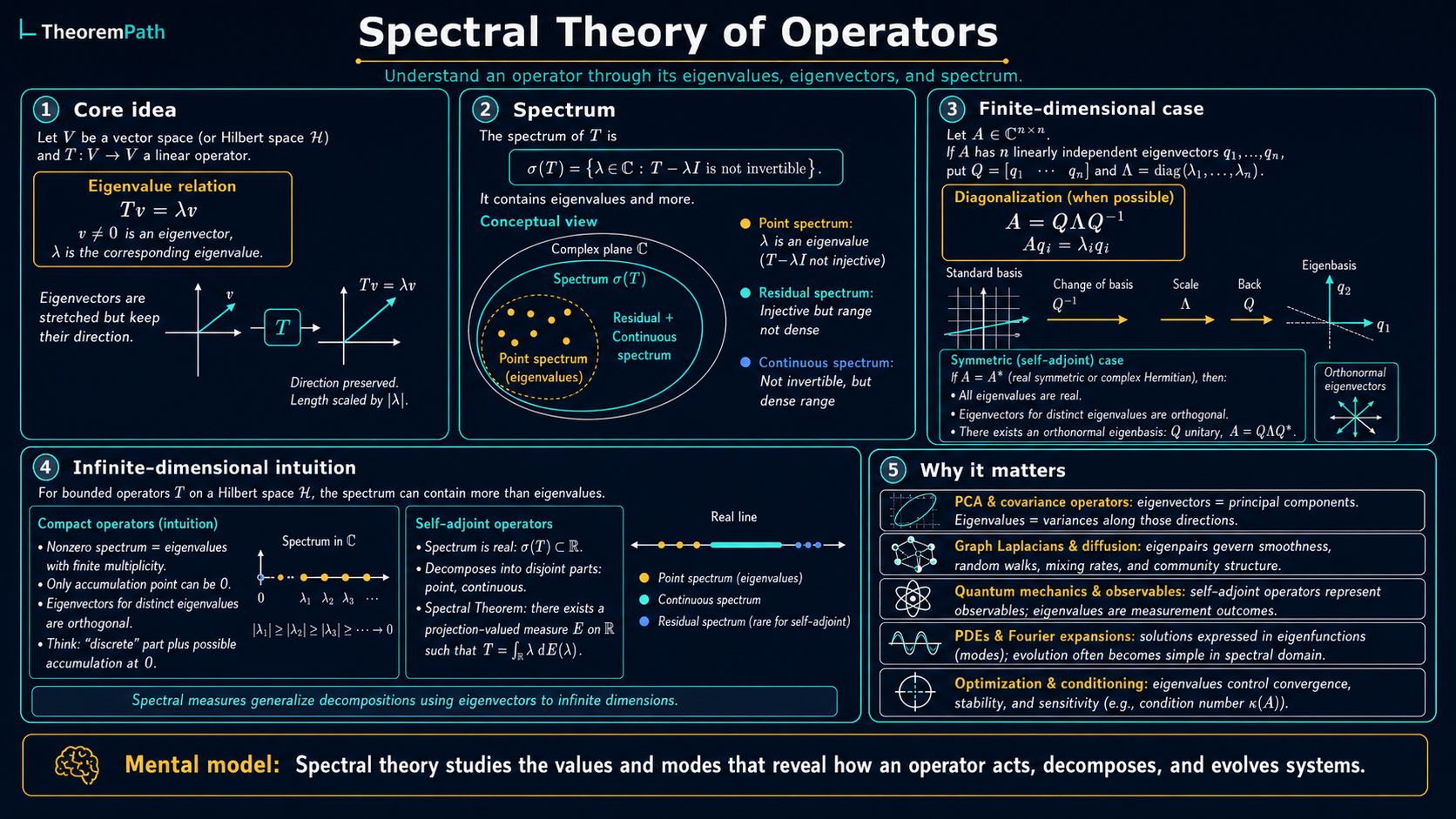
Spectral theorem for compact self-adjoint operators on Hilbert spaces: every such operator has a countable orthonormal eigenbasis with real eigenvalues accumulating only at zero. This is the infinite-dimensional backbone of PCA, kernel methods, and neural tangent kernel theory.
Why This Matters
In finite dimensions, the spectral theorem for symmetric matrices gives you PCA: diagonalize the covariance matrix and read off the principal components via eigenvalues and eigenvectors. But many ML methods live in infinite-dimensional spaces. Kernel methods operate in a reproducing kernel Hilbert space. Gaussian processes define covariance operators on function spaces. The neural tangent kernel is an infinite-width limit operator. To rigorously analyze any of these, you need the spectral theorem in infinite dimensions.
Hide overviewShow overview
The result is remarkably clean: compact self-adjoint operators on Hilbert spaces behave almost exactly like symmetric matrices, with a countable orthonormal eigenbasis and real eigenvalues.
Mental Model
A compact self-adjoint operator on a Hilbert space is the infinite-dimensional analog of a real symmetric matrix. Think of as stretching space along orthogonal directions (eigenfunctions) by amounts (eigenvalues) that decay to zero. The eigenvalues form a sequence converging to zero, and the eigenfunctions form a complete orthonormal basis for the range of .
The key difference from finite dimensions: the spectrum can have a continuous part in general, but compactness forces it to be discrete (except possibly at zero).
Formal Setup and Notation
Let be a separable Hilbert space with inner product . An operator is self-adjoint if and only if for all . It is compact if and only if it maps bounded sets to precompact sets (sets with compact closure).
Compact Operator
An operator is compact if and only if for every bounded sequence , the sequence has a convergent subsequence. Equivalently, is the norm limit of finite-rank operators. In ML: integral operators defined by continuous kernels on compact domains are compact.
Rayleigh Quotient
The Rayleigh quotient of a self-adjoint operator at is:
The supremum of over all nonzero equals the largest eigenvalue (or the supremum of the spectrum). This is the infinite-dimensional analog of the variational characterization of eigenvalues.
Main Theorems
Spectral Theorem for Compact Self-Adjoint Operators
Statement
Let be a compact self-adjoint operator on a separable Hilbert space. Then there exists a countable (finite or infinite) orthonormal sequence of eigenvectors with corresponding real eigenvalues such that:
The eigenvalues satisfy and if the sequence is infinite. The eigenvectors form an orthonormal basis for .
Intuition
A compact self-adjoint operator is a "matrix" with countably many rows and columns, all orthogonal, with entries (eigenvalues) that decay to zero. You can truncate the sum after terms to get a rank- approximation, just like truncated SVD in finite dimensions.
Proof Sketch
Step 1: Show , so either or is achieved (by compactness of the unit ball image). Step 2: The maximizer is an eigenvector with eigenvalue . Step 3: maps to itself (by self-adjointness), and the restriction is again compact and self-adjoint. Step 4: Induct to extract . Step 5: The remaining eigenvalues converge to zero by compactness.
Why It Matters
This theorem is the foundation of kernel PCA, Mercer's theorem, and the analysis of integral operators. When you compute the eigendecomposition of a kernel matrix, you are approximating this spectral decomposition. The decay rate of the eigenvalues determines the effective dimensionality of the RKHS and the statistical difficulty of kernel learning.
Failure Mode
Without compactness, the conclusion of the spectral theorem in this "countable eigenvalues converging to zero" form fails. The identity operator on a separable infinite-dimensional Hilbert space has spectrum and every nonzero vector is an eigenvector with eigenvalue , so it does admit an orthonormal eigenbasis — just not one whose eigenvalues decay to zero, which is exactly the property compactness would force. More general bounded self-adjoint operators (e.g. multiplication by on ) have purely continuous spectrum and no eigenvectors at all. Without self-adjointness, eigenvalues can be complex and eigenvectors need not be orthogonal.
Min-Max Characterization of Eigenvalues (Courant-Fischer)
Statement
The -th eigenvalue of a compact self-adjoint operator (in decreasing order) satisfies:
Intuition
The -th eigenvalue is the best worst-case Rayleigh quotient over all -dimensional subspaces. This gives a variational characterization that does not require knowing the previous eigenvectors. It directly implies that eigenvalues are stable under perturbations (Weyl's inequality).
Proof Sketch
For the max-min form: any -dimensional subspace must intersect nontrivially (by dimension counting). On this intersection, . Choosing achieves equality.
Why It Matters
The min-max principle is the theoretical foundation of PCA optimality. It proves that the top- eigenvectors give the best rank- subspace for capturing variance. It also gives eigenvalue perturbation bounds (Weyl's inequality) that control how eigenvalues change when the operator is perturbed.
Failure Mode
The min-max principle applies to self-adjoint operators. For non-self-adjoint operators (e.g., non-symmetric kernel matrices), singular values replace eigenvalues and the characterization involves both left and right subspaces.
The spectral theory here underpins the concentration inequalities used in kernel learning theory, where eigenvalue decay controls the effective complexity of the hypothesis class.
Connection to ML
Mercer's Theorem (Connection)
If is a continuous positive definite kernel on a compact domain, the integral operator is compact and self-adjoint. The spectral theorem gives . This is Mercer's theorem. The eigenfunctions are the feature map, and controls the importance of each feature.
Operator Classes and Spectral Structure
Hilbert-Schmidt and trace-class operators
A compact operator is Hilbert-Schmidt if and only if , equivalently . It is trace-class if and only if (using singular values in the non-self-adjoint case). The containments are strict: trace-class Hilbert-Schmidt compact. Mercer kernels with induce Hilbert-Schmidt integral operators, and continuous Mercer kernels on compact domains are trace-class with .
Singular value decomposition for compact operators
For a compact operator (not necessarily self-adjoint), there exist orthonormal systems in and in and non-negative singular values such that . The are the eigenvalues of . This is the exact parallel of the finite-dimensional SVD and reduces to the spectral theorem when is self-adjoint (with ).
Weyl's inequality
For self-adjoint compact operators with eigenvalues arranged in decreasing order, . This is the foundational spectral perturbation result: small additive perturbations produce small eigenvalue shifts. It follows directly from the Courant-Fischer min-max characterization.
Schatten -norms
For a compact operator with singular values , the Schatten -norm is for , with recovering the operator norm. is the trace class, is the Hilbert-Schmidt class (a Hilbert space under ). The Schatten classes are dual: with , paralleling the duality.
Canonical Examples
Spectral decomposition of a Gaussian kernel operator
Consider the Gaussian kernel on . The integral operator has eigenvalues that decay exponentially fast: . This rapid decay means the RKHS is effectively finite-dimensional, explaining why Gaussian kernel methods work well even with moderate sample sizes. The eigenfunctions resemble Hermite functions. This rate is exact on with Gaussian measure via Mehler's formula. On bounded domains with Lebesgue measure the decay is super-algebraic with a bandwidth-dependent rate (Santin-Schaback 2016 arXiv:1504.02868).
NTK spectral analysis
The neural tangent kernel at infinite width defines a compact self-adjoint operator on . The eigenvalue decay rate of this NTK operator determines the learning speed of gradient descent: modes with large eigenvalues are learned first, and modes with small eigenvalues are learned slowly or not at all. This is the spectral bias of neural networks.
Common Confusions
Bounded does not mean compact
Every compact operator is bounded, but not conversely. The identity operator on an infinite-dimensional Hilbert space is bounded but not compact. The compactness condition is strictly stronger and is what forces the eigenvalues to form a discrete sequence converging to zero.
Zero can be in the spectrum without being an eigenvalue
For compact operators, zero may or may not be an eigenvalue, but it is always in the spectrum when the Hilbert space is infinite-dimensional. The null space of (eigenvectors for eigenvalue 0) can be trivial, finite, or infinite-dimensional.
The empirical kernel matrix is not the operator
Training-time analysis often works with the Gram matrix , whose eigenvalues scale with and whose eigenvectors are vectors in . The underlying object is the integral operator on , whose eigenvalues are fixed and whose eigenfunctions are functions on . The two are linked by concentration: under mild conditions, with rate controlled by kernel smoothness (Koltchinskii-Giné 2000). When people write "kernel eigenvalue decay", they usually mean the operator eigenvalues; the matrix eigenvalues are only a finite-sample proxy.
Summary
- Compact self-adjoint operators have countable eigenvalues converging to zero
- Eigenvectors form an orthonormal basis for the closure of the range
- Rayleigh quotient variational principle gives eigenvalues without knowing eigenvectors
- Courant-Fischer min-max theorem implies PCA optimality and perturbation bounds
- Mercer's theorem connects kernel functions to spectral decompositions
- Eigenvalue decay rate controls effective dimensionality and learning difficulty
Exercises
Problem
Let be a compact self-adjoint operator with eigenvalues . Show that the best rank- approximation to in operator norm is and the approximation error is .
Problem
Suppose a kernel on has eigenvalues for . What is the trace of the integral operator ? What does this represent in terms of the kernel?
References
Canonical:
- Reed & Simon, Methods of Modern Mathematical Physics I: Functional Analysis (1980), Chapter VI
- Lax, Functional Analysis (2002), Chapters 28-31
Current:
- Steinwart & Christmann, Support Vector Machines (2008), Chapter 4 (Mercer's theorem for ML)
- Wainwright, High-Dimensional Statistics (2019), Chapter 12 (kernel operators)
- Santin & Schaback, "Approximation of eigenfunctions in kernel-based spaces" (2016), arXiv:1504.02868 (eigenvalue decay rates for Gaussian kernels on bounded domains)
Further directions
- Polar decomposition for non-self-adjoint operators
- Resolvent and functional calculus
- Stone's theorem for unbounded self-adjoint operators
- Spectral theorem for normal operators (broader class)
- Connection to empirical PCA and SVD of data matrix
- Kotani-Simon theorem on eigenvalue decay for Hilbert-Schmidt kernels
Next Topics
Natural extensions from spectral theory:
- Kernels and RKHS: reproducing kernel Hilbert spaces built on Mercer's theorem
- Neural tangent kernel: spectral analysis of infinite-width neural networks
- Principal component analysis: finite-sample spectral methods
- Functional analysis core: Hahn-Banach, open mapping, Banach-Alaoglu — the big four supporting all of this
Last reviewed: April 18, 2026
Canonical graph
Required before and derived from this topic
These links come from prerequisite edges in the curriculum graph. Editorial suggestions are shown here only when the target page also cites this page as a prerequisite.
Required prerequisites
3- Eigenvalues and Eigenvectorslayer 0A · tier 1
- Complex Numbers for Fourierlayer 0A · tier 2
- Functional Analysis Corelayer 0B · tier 2
Derived topics
2- DeepONetlayer 3 · tier 2
- Fourier Neural Operatorlayer 3 · tier 2
Graph-backed continuations