Foundations
Total Variation Distance
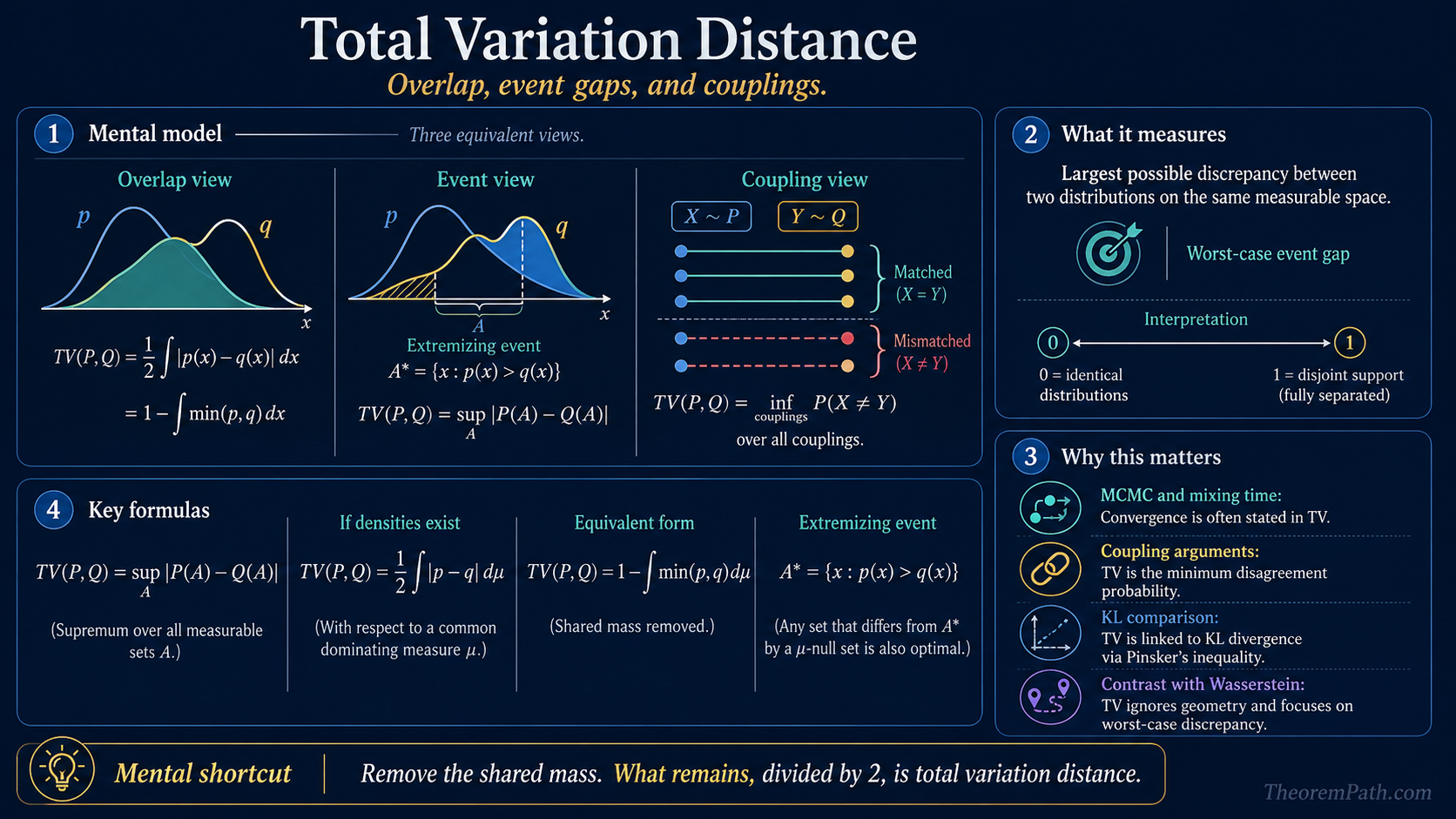
Total variation distance measures the largest possible discrepancy between two probability distributions: equivalently half the L1 gap, one minus the overlap mass, or the minimum disagreement probability under a coupling.
Why This Matters
Total variation distance is one of the standard notions of worst-case distributional discrepancy. If you give two models the freedom to disagree on any measurable event, total variation is the biggest probability gap they can produce.
Hide overviewShow overview
That single quantity shows up everywhere:
- in coupling arguments, where TV is the disagreement probability under the best joint construction
- in KL divergence, via Pinsker's inequality
- in Wasserstein distance, as the contrast case where geometry is ignored
- in MCMC and mixing-time theory, where convergence is often stated directly in TV
Mental Model
Three equivalent readings are worth holding at once:
- Overlap view. Remove the shared mass ; what remains is TV.
- Event view. Let an adversary pick the measurable set where the two distributions disagree most. The biggest gap is TV.
- Coupling view. Draw and on the same probability space in the smartest possible way. The smallest possible probability that is TV.
Each view is mathematically equivalent, but each teaches a different instinct.
Core Definitions
Total Variation Distance
For two probability measures and on the same measurable space,
The supremum runs over all measurable sets .
When densities and exist with respect to a common dominating measure, this becomes
So TV is literally half the distance, or equivalently one minus the overlap mass.
Main Theorems
Equivalent Forms of Total Variation
Statement
The following are equivalent:
If and are densities, the extremizing event is
Intuition
The signed difference has positive and negative regions. If you want the biggest possible probability gap, you keep exactly the region where exceeds and ignore the region where it falls below. That converts the absolute-value integral into the measurable-event supremum.
Proof Sketch
Split the space into and its complement. On , the difference is positive; on the complement, it is negative. Therefore
This gives . The overlap identity follows from the pointwise equality and the fact that .
Why It Matters
This theorem is why TV is so interpretable. It is simultaneously an adversarial event gap, a density-overlap deficit, and an discrepancy. Different subfields pick different forms, but they are all the same object.
Failure Mode
TV ignores geometry. Two point masses at nearby locations can have even if the ambient metric says they are extremely close. That is exactly why Wasserstein distance exists.
Coupling Characterization of Total Variation
Statement
Among all couplings with marginals and ,
Moreover, there exists a maximal coupling attaining equality.
Intuition
The common overlap mass can be coupled to agree exactly. Only the leftover unmatched mass must disagree. So the best possible disagreement probability is precisely the amount of unmatched mass, which is TV.
Proof Sketch
Write the shared mass as . Sample from the normalized overlap and set there. The remaining residual masses of and are then sampled independently on the non-overlap part. Agreement happens exactly on the shared-mass component, whose total weight is . Hence the disagreement probability is .
Why It Matters
This is the bridge from abstract probability metrics to concrete stochastic processes. In mixing-time proofs, you often build a coupling and show the two chains have met by time with high probability; the theorem converts that meeting event directly into a TV bound.
Failure Mode
Not every naive coupling is maximal. A bad coupling can make the disagreement probability much larger than TV. The theorem says TV is the best possible disagreement rate, not the rate produced by an arbitrary coupling.
Pinsker's Inequality
TV and KL are linked by the classical bound
The constant assumes KL is measured in nats (natural log). If KL is measured in bits (), the bound becomes . Always check the log base before plugging in numbers.
This is useful in lower bounds, concentration arguments, and asymptotic statistics because KL often tensorizes more easily than TV. But it is only a one-way control: small KL implies small TV, while the reverse is false without extra assumptions.
There is no universal reverse Pinsker inequality
Small TV does not imply small KL in general. KL is unbounded — it can be infinite while TV is finite (and at most one). The standard counterexample: has support that includes a region where assigns zero mass; then but . Reverse Pinsker bounds exist only under extra conditions, e.g., a uniform bound on the likelihood ratio or a bounded chi-squared divergence. When you need both directions, state the regularity assumption that controls KL from above.
Worked Example: TV Between Two Gaussians
For and with , the densities cross at , and the optimal event is . The closed form is
where is the standard normal CDF. Numeric values:
| Mean shift | (Pinsker) | Slack: Pinsker TV | |
|---|---|---|---|
| 0.1 | 0.0398 | 0.0500 | 0.0102 |
| 0.5 | 0.1974 | 0.2500 | 0.0526 |
| 1.0 | 0.3829 | 0.5000 | 0.1171 |
| 2.0 | 0.6827 | 1.0000 | 0.3173 |
The KL between two unit-variance Gaussians with mean shift is , so Pinsker's bound says . The bound is tight at (both vanish at rate vs ) but loose for moderate-to-large . By , Pinsker overstates TV by 47%.
This is the canonical illustration of the slack in Pinsker. Tighter inequalities (Bretagnolle-Huber, refined Pinsker bounds) close some of this gap when needed.
Le Cam's Two-Point Method
TV is the central object in minimax lower bounds for hypothesis testing and parameter estimation. The mechanism is Le Cam's two-point inequality.
Le Cam's Two-Point Inequality
Statement
For any binary test distinguishing from ,
The minimum total error of any test is exactly , and the optimal test is the likelihood-ratio test thresholded at 1.
Intuition
Tests can only do as well as the distributions allow them to. The probability of correct discrimination is bounded by the overlap deficit. If , the two distributions are identical and no test can beat random guessing; if , the two distributions have disjoint support and a perfect test exists.
Why It Matters
Le Cam's method converts every minimax lower-bound problem into a TV computation. Pick two parameter values separated by . The minimax risk for any estimator is at least . To produce a non-trivial lower bound, pick small enough that the -fold TV stays bounded away from 1.
Failure Mode
The two-point method gives only a lower bound, often loose. For tighter rates, use Fano's inequality (multiple hypotheses) or Assouad's lemma (parameter-cube hypotheses). The two-point method is the simplest case and the foundation for all of them.
The TV-tensorization rule for product measures, (with equality only in the trivial cases), is what controls how much samples shrink the error rate. For , the error decays as , exponential in the number of samples.
Maximal Coupling: An Explicit Construction
The coupling theorem above guarantees a maximal coupling exists. Here is the explicit construction for densities on with respect to Lebesgue measure.
Let and . The procedure:
- Toss a coin with .
- If heads (probability ): sample and set .
- If tails (probability ): sample and independently.
Verify the marginals: with probability , has density , and with probability , has density . The mixture density is . Same for with marginal . The disagreement event occurs only on tails, with probability . Done.
For specific examples (two Gaussians, two Bernoullis, two Poissons), this construction is explicit and computable. It is the workhorse of mixing-time arguments for Markov chains: build a coupling, bound the meeting time, convert to TV.
Why TV and Wasserstein Feel Different
TV is a support-sensitive metric: if two distributions place mass on disjoint sets, TV is already maximal. Wasserstein is a geometry-sensitive metric: if those disjoint sets are close in the ambient space, Wasserstein can still be small.
This difference explains the common dichotomy:
- TV is natural for hypothesis testing, coupling, and mixing.
- Wasserstein is natural for transport, generative modeling, and robustness with geometric structure.
Common Confusions
TV is a metric, but it is not geometric
TV satisfies symmetry and the triangle inequality, so it is a genuine metric. But it does not know about ambient distances between outcomes. It only sees how much mass fails to overlap.
The factor 1/2 is convention, not substance
Some ML papers define TV as without the . Probability texts almost always include the , giving range . The two conventions differ by exactly a factor of two. Always check which one a paper uses before comparing constants.
Summary
- — adversarial event gap
- with densities,
- TV is the smallest disagreement probability over all couplings; the maximal coupling attaining it is explicitly constructible
- TV is sensitive to support mismatch but blind to geometry; Wasserstein is the geometric counterpart
- Pinsker links TV to KL: , tight as , loose for moderate-to-large
- For vs :
- Le Cam's two-point method: minimax test error
- TV product-tensorization: (linear, useless once ); Bretagnolle-Huber gives exponential control instead
Exercises
Problem
Let and . Compute using both the event-gap definition and the formula.
Problem
Verify Pinsker's inequality for and for small . Compute exactly and compare to .
Problem
Let and be the -fold product measures of and . Show that . Explain why this bound, while linear in , becomes useless as soon as .
References
Canonical:
- Levin, D. A., Peres, Y., & Wilmer, E. L. (2009). Markov Chains and Mixing Times. AMS. Chapter 4 is the standard reference for TV in mixing-time arguments and the coupling construction.
- Villani, C. (2009). Optimal Transport: Old and New. Springer. Chapter 6 covers the contrast between TV and Wasserstein and explains why the geometric/non-geometric distinction matters.
- Le Cam, L. (1986). Asymptotic Methods in Statistical Decision Theory. Springer. The original treatment of the two-point method and TV's role in minimax theory.
- Lindvall, T. (1992). Lectures on the Coupling Method. Wiley. The classical treatment of coupling theory; chapters 1-2 cover TV and the maximal coupling.
Current / standard texts:
- Durrett, R. (2019). Probability: Theory and Examples (5th ed.). Cambridge University Press. Sections on coupling and total variation in the discrete-time chain chapters.
- van der Vaart, A. W. (1998). Asymptotic Statistics. Cambridge University Press. Appendix and Chapter 7 cover TV-KL relations in the M-estimation context.
- Wainwright, M. J. (2019). High-Dimensional Statistics: A Non-Asymptotic Viewpoint. Cambridge University Press. Chapter 3 covers TV, KL, and chi-squared divergences in the modern non-asymptotic setting.
- Polyanskiy, Y., & Wu, Y. (2025). Information Theory: From Coding to Learning. Cambridge University Press. Chapter 7 covers -divergences (TV, KL, chi-squared) with refined Pinsker-style inequalities and a unified Le-Cam-type framework.
Refined inequalities:
- Bretagnolle, J., & Huber, C. (1979). Estimation des densités: risque minimax. Zeitschrift für Wahrscheinlichkeitstheorie, 47(2), 119-137. The Bretagnolle-Huber inequality , which is tighter than Pinsker for large KL.
Last reviewed: May 4, 2026
Canonical graph
Required before and derived from this topic
These links come from prerequisite edges in the curriculum graph. Editorial suggestions are shown here only when the target page also cites this page as a prerequisite.
Required prerequisites
2- Common Probability Distributionslayer 0A · tier 1
- Measure-Theoretic Probabilitylayer 0B · tier 1
Derived topics
3- KL Divergencelayer 1 · tier 1
- Coupling Arguments and Mixing Timelayer 3 · tier 3
- Wasserstein Distanceslayer 4 · tier 3
Graph-backed continuations