Gibbs Sampling

Why This Matters

Gibbs sampling is a foundational MCMC algorithm with a long history in applied Bayesian statistics. It powered earlier-generation tools like BUGS and JAGS, and remains standard whenever a model has full conditionally conjugate structure. Modern general-purpose Bayesian workflows more often reach for Hamiltonian Monte Carlo (Stan defaults to NUTS) because Gibbs mixes poorly in high-dimensional or strongly correlated posteriors. Gibbs still wins when the conditionals are closed-form: hierarchical models with conjugate priors, mixture models, LDA-style latent-variable models, and any setting where sampling from $p(x_i \mid x_{-i})$ is cheap.

Hide overviewShow overview

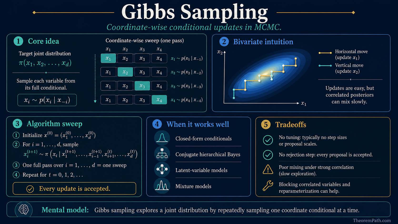
Its appeal is simplicity: instead of designing a proposal distribution and tuning acceptance rates, you just sample each variable from its conditional distribution given the rest. No tuning parameters, no rejections.

Mental Model

The target is a joint distribution π$(x_1, \ldots, x_d)$ that is hard to sample from directly. The full conditionals $\pi(x_i \mid x_{-i})$ are often tractable when the joint is not, for example in Bayesian models with conjugate priors, where each $x_i \mid x_{-i}$ reduces to a standard distribution.

Gibbs sampling cycles through the coordinates, drawing each $x_i$ from its full conditional given the current values of the others. The resulting Markov chain has $\pi$ as its stationary distribution.

Formal Setup and Notation

Let $\pi(x_1, x_2, \ldots, x_d)$ be the target joint distribution. We assume we can sample from each full conditional distribution.

Definition

Full Conditional Distribution$\pi (x_i\mid x_{-i})$

The full conditional distribution of variable $x_i$ given all other variables is:

$\pi(x_i \mid x_{-i}) = \pi(x_i \mid x_1, \ldots, x_{i-1}, x_{i+1}, \ldots, x_d) = \frac{\pi(x_1, \ldots, x_d)}{\int \pi(x_1, \ldots, x_d)\, dx_i}$

where $x_{-i}$ denotes all variables except $x_i$. In practice, to derive the full conditional for $x_i$, you write out the full joint density, treat everything that does not involve $x_i$ as a constant, and recognize the resulting kernel as a known distribution.

Definition

Gibbs Sampler (Systematic Scan)

Given target $\pi(x_1, \ldots, x_d)$ and initial state $(x_1^{(0)}, \ldots, x_d^{(0)})$:

At iteration $t$, update each component in sequence:

1. Draw $x_1^{(t)} \sim \pi(x_1 \mid x_2^{(t-1)}, x_3^{(t-1)}, \ldots, x_d^{(t-1)})$
2. Draw $x_2^{(t)} \sim \pi(x_2 \mid x_1^{(t)}, x_3^{(t-1)}, \ldots, x_d^{(t-1)})$
3. Continue through all variables...
4. Draw $x_d^{(t)} \sim \pi(x_d \mid x_1^{(t)}, x_2^{(t)}, \ldots, x_{d-1}^{(t)})$

Note: each update uses the most recent values of all other variables.

Definition

Random Scan Gibbs Sampler

An alternative to systematic scan: at each iteration, choose an index $i \in \{1, \ldots, d\}$ uniformly at random (or with specified probabilities), and update only $x_i$ from $\pi(x_i \mid x_{-i})$.

Random scan has cleaner theoretical properties (it satisfies detailed balance directly), while systematic scan is more commonly used in practice because it updates all variables every iteration.

Gibbs as a Special Case of Metropolis-Hastings

The central theoretical result about Gibbs sampling is that it is a special case of MH where the acceptance probability is always 1.

Theorem

Gibbs Sampling Has Acceptance Probability 1

Statement

Consider a single Gibbs update for variable $x_i$: propose $x_i'$ from $\pi(x_i' \mid x_{-i})$. This is equivalent to a Metropolis-Hastings step with proposal $q(x_i' \mid x_i, x_{-i}) = \pi(x_i' \mid x_{-i})$ and acceptance probability:

$\alpha = \min\!\left(1,\;\frac{\pi(x_i', x_{-i})\, \pi(x_i \mid x_{-i})}{\pi(x_i, x_{-i})\, \pi(x_i' \mid x_{-i})}\right) = 1$

Every proposed move is accepted.

Intuition

The proposal distribution is exactly the full conditional. The optimal distribution for $x_i$ given everything else. There is no mismatch between proposal and target to correct for, so the acceptance ratio evaluates to 1. You are proposing from exactly the right distribution.

Proof Sketch

By definition of the full conditional: $\pi(x_i, x_{-i}) = \pi(x_i \mid x_{-i})\,\pi(x_{-i})$.

The acceptance ratio becomes:

$\alpha = \frac{\pi(x_i' \mid x_{-i})\,\pi(x_{-i}) \cdot \pi(x_i \mid x_{-i})}{\pi(x_i \mid x_{-i})\,\pi(x_{-i}) \cdot \pi(x_i' \mid x_{-i})} = \frac{\pi(x_{-i})}{\pi(x_{-i})} = 1$

The $\pi(x_i \mid x_{-i})$ and $\pi(x_{-i})$ terms cancel perfectly.

Why It Matters

A single Gibbs update is a valid MH step with acceptance probability 1, so it preserves $\pi$ as the stationary distribution and avoids proposal tuning and rejected samples. The full guarantees, however, depend on the scan type: random-scan Gibbs is reversible (satisfies detailed balance with respect to $\pi$) and is most directly an MH kernel; systematic-scan Gibbs preserves $\pi$ as a composition of MH kernels but is generally only $\pi$-invariant and not reversible. Convergence in either case still requires the standard Markov-chain assumptions on top of $\pi$-invariance: $\pi$-irreducibility, Harris recurrence on general state spaces, aperiodicity where relevant, and connected positive-density support of $\pi$. Compatibility of the full conditionals (a single joint $\pi$ that realizes them all) is implicit and matters in practice.

Failure Mode

The acceptance rate of 1 does not mean Gibbs sampling is always efficient. The chain can still mix slowly if the variables are highly correlated. When $x_1$ and $x_2$ are strongly correlated, updating one at a time while fixing the other leads to slow, diffusive exploration. The chain takes small steps along the correlation ridge. This is the main weakness of component-wise Gibbs sampling.

report a correction →

Theorem

Convergence of the Gibbs Sampler

Statement

Under mild regularity conditions, the Gibbs sampler is ergodic: starting from any initial state $x^{(0)}$, the distribution of $x^{(t)}$ converges to $\pi$ in total variation:

$\lim_{t \to \infty} \|P^t(x^{(0)}, \cdot) - \pi(\cdot)\|_{\text{TV}} = 0$

For random scan, the chain satisfies detailed balance with respect to $\pi$. For systematic scan, the chain satisfies the weaker condition of $\pi$-invariance (but not necessarily detailed balance).

Intuition

Each Gibbs update preserves $\pi$ as the stationary distribution (since it is a valid MH step). As long as the chain can reach any state, guaranteed when the support is connected and the full conditionals have positive density, the chain converges. Random scan gives reversibility automatically; systematic scan gives faster practical convergence but sacrifices reversibility.

Proof Sketch

For random scan: the transition kernel is a mixture of MH kernels, each satisfying detailed balance, so the mixture does too. Irreducibility follows from the positivity of full conditionals on the support.

For systematic scan: the transition kernel is a composition (not mixture) of MH kernels. Each kernel preserves $\pi$, so the composition does too. Detailed balance may fail, but $\pi$-invariance plus irreducibility and aperiodicity suffice for convergence.

Why It Matters

This theorem ensures that Gibbs sampling produces valid samples from the target distribution, justifying its use in Bayesian computation. The distinction between random and systematic scan matters for theoretical analysis (e.g., proving CLTs for MCMC estimators) but rarely affects practice.

Failure Mode

Convergence can be extremely slow when variables are strongly correlated or when the posterior has multiple well-separated modes. In the latter case, the chain may get trapped in one mode for a very long time. Blocking (grouping correlated variables and updating them jointly) can help with correlations; tempering or other advanced methods are needed for multimodality.

report a correction →

Blocking for Correlated Variables

When variables $x_i$ and $x_j$ are highly correlated, updating them one at a time leads to slow mixing. Blocking (or collapsed Gibbs) groups correlated variables together and samples them jointly:

Instead of updating $x_1 \mid x_2, x_3$ then $x_2 \mid x_1, x_3$, update $(x_1, x_2) \mid x_3$ as a block. This requires sampling from the joint conditional $\pi(x_1, x_2 \mid x_3)$, which may itself require specialized methods, but the resulting chain mixes much faster when $x_1$ and $x_2$ are correlated.

The general principle: block together variables that are strongly correlated a posteriori.

Diagnostics Matter Even When Every Proposal Is Accepted

The most seductive Gibbs-sampling mistake is to see a 100% acceptance rate and infer that the sampler must be efficient. It is not. Gibbs can accept every single update and still produce a terrible effective sample size.

That happens when the conditional updates move only a tiny distance along a strong posterior ridge. The bivariate normal example above shows the core mechanism: when $|\rho|$ is close to 1, the conditional variance shrinks and each update becomes a small creep rather than a meaningful exploration move. The result is high autocorrelation, which makes the effective sample size much smaller than the chain length suggests.

So the right workflow is:

• derive the conditionals cleanly,
• run multiple chains,
• inspect burn-in and convergence diagnostics,
• and if ESS remains poor, change the geometry of the update, not just the iteration count.

For hierarchical models this often means blocking, collapsing, or changing the parameterization itself.

Hierarchical Models: Centered, Non-Centered, and Conjugacy

Gibbs sampling has a special relationship to hierarchical models. In one direction, it is often the easiest exact MCMC method when the hierarchy is conditionally conjugate: normal-normal random effects, Gaussian state-space models, latent-class assignments, and older BUGS/JAGS workflows all lean on that structure.

But there is a catch. The parameterization that is best for Gibbs is not always the one that is best for HMC or NUTS.

• A centered hierarchy often preserves clean conditional conjugacy, so the Gibbs updates stay closed-form.
• A non-centered hierarchy often reduces posterior correlation between local effects and the global scale, which is better geometry for HMC and NUTS, but may destroy the simple conditional form that made Gibbs attractive in the first place.

So "use the non-centered form" is not a universal rule. It is a rule about a particular geometry-sampler pairing. For the full comparison, see Centered vs. Non-Centered Hierarchical Models.

Gibbs for Conjugate Models

The power of Gibbs sampling is most apparent in conjugate models, where each full conditional belongs to a standard distribution family.

Example

Normal-Normal model (known variance)

Model: $x_i \mid \mu \sim \mathcal{N}(\mu, \sigma^2)$ for $i=1,\ldots,n$, with prior $\mu \sim \mathcal{N}(\mu_0, \tau^2)$.

The full conditional for $\mu$ is:

$\mu \mid x_1, \ldots, x_n \sim \mathcal{N}\!\left(\frac{n\bar{x}/\sigma^2 + \mu_0/\tau^2}{n/\sigma^2 + 1/\tau^2},\; \frac{1}{n/\sigma^2 + 1/\tau^2}\right)$

This is a one-block model, so one Gibbs draw gives an exact posterior sample. The power of Gibbs becomes clear in hierarchical extensions with additional latent variables.

Example

Beta-Binomial model

Model: $x \mid \theta \sim \text{Binomial}(n, \theta)$, with prior $\theta \sim \text{Beta}(\alpha, \beta)$.

The full conditional is:

$\theta \mid x \sim \text{Beta}(\alpha + x, \beta + n - x)$

Again conjugacy gives a closed-form full conditional. In a hierarchical model with multiple groups sharing a common prior, the Gibbs sampler alternates between updating group-level parameters and the hyperparameters.

Example

Gibbs for a bivariate normal

Target: $(x_1, x_2) \sim \mathcal{N}\!\left(\begin{pmatrix}0\\0\end{pmatrix}, \begin{pmatrix}1 & \rho\\ \rho & 1\end{pmatrix}\right)$.

The full conditionals are:

$x_1 \mid x_2 \sim \mathcal{N}(\rho\, x_2,\; 1 - \rho^2)$ $x_2 \mid x_1 \sim \mathcal{N}(\rho\, x_1,\; 1 - \rho^2)$

When $|\rho|$ is close to 1, the chain moves in small steps along the diagonal, illustrating the slow-mixing problem for correlated variables. The autocorrelation of the chain is approximately $\rho^2$ per iteration.

Common Confusions

Watch Out

Gibbs requires KNOWN full conditionals

Gibbs sampling requires that you can derive and sample from each full conditional distribution. If the full conditional does not have a recognizable closed form, you cannot use standard Gibbs for that variable. The solution is MH within Gibbs: use a Metropolis-Hastings step (with some proposal distribution) to update that variable, while using exact Gibbs updates for the variables where full conditionals are known. This hybrid approach is extremely common in practice.

Watch Out

Gibbs is not always better than MH

The 100% acceptance rate of Gibbs does not mean it is always more efficient than MH. In high-correlation scenarios, a well-tuned MH proposal that accounts for correlations (or Hamiltonian Monte Carlo, which uses gradient information) can vastly outperform component-wise Gibbs. Gibbs excels when the model has conditionally conjugate structure and moderate correlations.

Watch Out

Acceptance probability 1 does not mean i.i.d. draws

Every Gibbs proposal is accepted because it is drawn from the correct full conditional. That says nothing about how correlated successive full states are. A Gibbs chain can have severe autocorrelation and a tiny effective sample size even though the acceptance rate is exactly 1.

Watch Out

Systematic scan Gibbs does not satisfy detailed balance

A common misconception is that Gibbs sampling always satisfies detailed balance. In fact, only random scan Gibbs satisfies detailed balance. Systematic scan Gibbs, where you cycle through variables in a fixed order, satisfies the weaker property of $\pi$-invariance: $\pi K = \pi$ where $K$ is the transition kernel. This is sufficient for convergence but means some theoretical tools (e.g., certain CLT results) require more care.

Watch Out

Gibbs updates use the MOST RECENT values

In systematic scan, when updating $x_i$, you condition on the values of $x_1, \ldots, x_{i-1}$ that have already been updated in the current iteration, and the values of $x_{i+1}, \ldots, x_d$ from the previous iteration. This is not the same as conditioning on all values from the previous iteration (which would be a different, valid but less efficient, algorithm sometimes called "synchronous" or "parallel" Gibbs).

Summary

• Gibbs sampling updates each variable from its full conditional, cycling through all variables
• It is a special case of MH with acceptance probability 1
• Requires known, tractable full conditional distributions
• Random scan satisfies detailed balance; systematic scan only satisfies $\pi$-invariance
• Excels in conditionally conjugate models and older hierarchical Bayesian workflows
• Blocking, collapsing, and parameterization matter because 100% acceptance does not guarantee good ESS
• When full conditionals are not tractable, use MH within Gibbs or move to a geometry-aware method like HMC

Exercises

ExerciseCore

Problem

Derive the Gibbs sampler for the bivariate normal distribution:

$(x_1, x_2) \sim \mathcal{N}\!\left(\begin{pmatrix}\mu_1\\\mu_2\end{pmatrix}, \begin{pmatrix}\sigma_1^2 & \rho\sigma_1\sigma_2\\ \rho\sigma_1\sigma_2 & \sigma_2^2\end{pmatrix}\right)$

Find both full conditional distributions $\pi(x_1 \mid x_2)$ and $\pi(x_2 \mid x_1)$.

Hint

Reveal Solution

ExerciseCore

Problem

Prove that the Gibbs update for variable $x_i$, viewed as an MH step with proposal $q(x_i' \mid x_i, x_{-i}) = \pi(x_i' \mid x_{-i})$, has acceptance probability exactly 1.

Hint

Reveal Solution

ExerciseAdvanced

Problem

Consider a mixture model: $x_i \mid z_i, \mu_1, \mu_2 \sim \mathcal{N}(\mu_{z_i}, 1)$ with $z_i \in \{1, 2\}$, $P(z_i = 1) = 0.5$, and priors $\mu_k \sim \mathcal{N}(0, 10)$. Derive the full conditional distributions for the Gibbs sampler: $\pi(z_i \mid \text{rest})$ and $\pi(\mu_k \mid \text{rest})$.

Hint

Reveal Solution

References

Canonical:

• Geman & Geman (1984), "Stochastic Relaxation, Gibbs Distributions, and the Bayesian Restoration of Images"
• Gelfand & Smith (1990), "Sampling-Based Approaches to Calculating Marginal Densities"
• Casella & George (1992), "Explaining the Gibbs Sampler," The American Statistician 46(3), 167-174. Still one of the cleanest expositions of why the algorithm works.

Current:

• Robert & Casella, Monte Carlo Statistical Methods (2004), Chapter 10
• Gelman, Carlin, Stern, Dunson, Vehtari, Rubin, Bayesian Data Analysis (3rd ed., 2013), Chapter 11
• Brooks et al., Handbook of MCMC (2011), Chapters 1-5
• Betancourt & Girolami, "Hamiltonian Monte Carlo for Hierarchical Models" (2013, arXiv:1312.0906). Useful contrast for when conditional conjugacy stops being the dominant consideration.

Next Topics

The natural next steps from Gibbs sampling:

• Griddy Gibbs: approximate Gibbs when full conditionals are not available in closed form
• Burn-in and Convergence Diagnostics: how to assess whether the chain has converged and whether ESS is actually usable
• Hamiltonian Monte Carlo: when gradient-guided global moves beat component-wise conditional updates
• Centered vs. Non-Centered Hierarchical Models: when the best parameterization for Gibbs is not the best one for NUTS