Sampling MCMC
Hamiltonian Monte Carlo
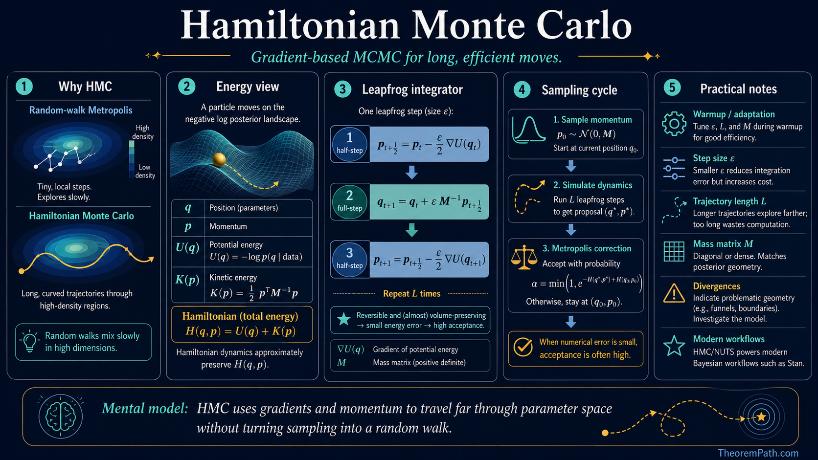
HMC uses gradients and Hamiltonian dynamics to propose large moves that still land in high-density regions. The real practical story includes leapfrog geometry, warmup, divergences, and when centered hierarchical models break the sampler.
Why This Matters
Metropolis-Hastings (MH) with a random walk proposal is the simplest MCMC algorithm, but it fails in high dimensions. The random walk takes tiny steps to maintain a reasonable acceptance rate, resulting in extremely slow exploration. In the canonical analysis of Roberts, Gelman, Gilks (1997) for product-form target distributions, the cost of one effective sample under random-walk MH scales as in dimension . For even moderate this is prohibitively slow under that analysis, and the empirical picture is similar for many smooth high-dimensional posteriors.
Hide overviewShow overview
Hamiltonian Monte Carlo (HMC) solves this by using gradient information to propose distant points in parameter space that are still likely to be accepted. The companion analysis (Beskos, Pillai, Roberts, Sanz-Serna, Stuart 2013) shows that the cost of one effective sample under HMC scales as for the same product-form targets. These exponents are reference rates derived for product-form targets in the diffusion limit, not universal mixing-time guarantees. They predict the right qualitative ordering on a broad range of smooth posteriors, which is why Bayesian inference in hundreds or thousands of dimensions is practical with HMC, but worst-case mixing times for non-log-concave or geometrically pathological targets can be much worse.
HMC is the engine behind Stan, one of the most widely used probabilistic programming languages, and is the default MCMC algorithm for serious Bayesian modeling.
Mental Model
Imagine a ball rolling on a surface whose height at position is the . The ball naturally rolls toward regions of high posterior density (low ) and maintains to traverse ridges between modes.
HMC simulates this physics. Instead of randomly proposing a new point, it gives the current point a random "kick" (momentum) and then follows the laws of physics (Hamilton's equations) for a fixed time. The endpoint of this trajectory is the proposal. Because the trajectory follows the posterior landscape, the proposal tends to be in a region of similar density, even if it is far from the starting point.
Formal Setup and Notation
We want to sample from a target distribution with density where are the parameters and is the potential energy (up to a constant).
HMC introduces an auxiliary momentum variable on and defines the joint distribution:
where the Hamiltonian is:
The kinetic energy is typically , where is a mass matrix (often ). The marginal distribution of is the target , and .
Core Definitions
Hamilton's Equations
The Hamiltonian dynamics are governed by:
These equations describe how position and momentum evolve over time. The key property: the Hamiltonian is conserved along the trajectory. A particle moving along this trajectory stays on a contour of constant .
Leapfrog Integrator
Since we cannot solve Hamilton's equations analytically for general , we use a numerical integrator. The leapfrog (Stormer-Verlet) integrator with step size :
This is repeated times to produce the proposal. Each step requires one gradient evaluation .
HMC Algorithm
One iteration of HMC:
- Resample momentum: Draw
- Simulate dynamics: Starting from , run leapfrog steps with step size to get
- Negate momentum: Set (for reversibility)
- Metropolis accept/reject: Accept with probability
If the leapfrog integrator were exact (zero discretization error), the Hamiltonian would be perfectly conserved and the acceptance probability would be 1. In practice, the acceptance rate depends on and .
Main Theorems
Conservation Properties of Hamiltonian Dynamics
Statement
The exact Hamiltonian flow has three crucial properties:
- Energy conservation: for all .
- Volume preservation (Liouville's theorem): The flow preserves the Lebesgue measure on phase space .
- Reversibility: If is evolved for time , it returns to .
Together, these ensure that the dynamics leave the joint distribution invariant.
Intuition
Energy conservation means the proposal has the same Hamiltonian value as the starting point, so acceptance probability is 1. Volume preservation means we do not need a Jacobian correction in the acceptance probability. Reversibility ensures detailed balance. These three properties are exactly what we need for a valid MCMC proposal.
Why It Matters
These properties explain why HMC works. The Hamiltonian flow is a measure-preserving, reversible map on phase space that conserves energy. It is the ideal MCMC proposal: it moves you to a distant point with the same target density, guaranteed. The only reason we need the Metropolis-Hastings correction is that the leapfrog integrator introduces discretization error, breaking exact energy conservation.
Leapfrog Preserves Volume
Statement
The leapfrog integrator is a symplectic integrator: it preserves the symplectic 2-form on phase space. In particular, it is volume-preserving (the Jacobian of the leapfrog map has determinant 1) and time-reversible.
The local truncation error in the position variable is per step. More importantly, because leapfrog is symplectic, the energy error along the trajectory is bounded by uniformly in the number of steps (the error does not accumulate linearly, unlike non-symplectic integrators). This bounded-energy-error property comes from the shadow-Hamiltonian analysis (Hairer, Lubich, Wanner 2006).
Intuition
The leapfrog integrator inherits the volume-preservation and reversibility of exact Hamiltonian dynamics, even though it does not conserve energy exactly. This is why leapfrog is used instead of, say, Euler's method: Euler's method is neither volume-preserving nor reversible, and would require a Jacobian correction that is expensive to compute.
The non-accumulation of energy error is the key miracle: after steps, the Hamiltonian error is still , not . This is because the leapfrog trajectory stays on a "shadow Hamiltonian" that is -close to the true Hamiltonian.
Why It Matters
Volume preservation means the Metropolis acceptance probability is simply with no Jacobian term. Reversibility ensures detailed balance. The global error means we can take large steps (large ) while maintaining high acceptance rates, which is exactly what makes HMC efficient.
HMC Satisfies Detailed Balance
Statement
The HMC transition kernel satisfies detailed balance with respect to the joint distribution . Therefore, is a stationary distribution of the HMC Markov chain (marginalizing over ).
Intuition
The momentum resampling step leaves invariant because is drawn from its conditional . The leapfrog + Metropolis step leaves invariant because leapfrog is volume-preserving and reversible, and the Metropolis correction accounts for the energy error. Composing two -invariant steps gives a -invariant chain.
Why HMC Beats Random-Walk MH
The fundamental problem with random-walk MH in dimensions, under the product-target diffusion-limit analysis of Roberts, Gelman, Gilks (1997):
- To maintain acceptance rate (optimal), the step size must scale as .
- The chain takes steps of size , so it needs steps to traverse one standard deviation of the target.
- Total cost to get one effective sample: density evaluations.
HMC with properly tuned and , under the matching analysis of Beskos, Pillai, Roberts, Sanz-Serna, Stuart (2013):
- The leapfrog trajectory can traverse the entire target distribution in one proposal.
- The optimal step size scales as .
- Total cost per effective sample: gradient evaluations.
The improvement from to in this product-target regime is the canonical reason HMC is practical for high-dimensional Bayesian inference. The cost is requiring , which is not always available, and these scalings are not guaranteed for non-product or non-log-concave targets — multimodal posteriors, funnels, and posteriors with heavy tails or sharp ridges can mix much more slowly.
MCMC Sampler Comparison
The following table compares HMC against other MCMC methods across the dimensions that matter for practical Bayesian inference.
| Property | Random-walk MH | Gibbs sampling | HMC (NUTS) | Langevin MCMC |
|---|---|---|---|---|
| Cost per step | density eval | conditional evals | gradient evals | gradient eval |
| Scaling with | for one effective sample | (worse with correlation) | ||
| Requires gradients | No | No | Yes | Yes |
| Handles correlation | Poorly (slow mixing) | Poorly (blocked Gibbs helps) | Well (momentum carries through correlated dimensions) | Moderately |
| Tuning parameters | Proposal scale | Conditional distributions | , (NUTS auto-tunes both) | Step size only |
| Optimal acceptance rate | 0.234 | 1.0 (exact conditionals) | 0.65 (HMC) or 0.80 (NUTS) | 0.574 |
| Multimodal targets | Very slow | Very slow | Slow (cannot jump between modes) | Very slow |
When HMC Fails
HMC is not a universal solution. Several target distribution geometries cause problems.
Multimodal targets. HMC explores a single mode efficiently but cannot jump between well-separated modes. The Hamiltonian dynamics are continuous, so the trajectory must pass through the low-density region between modes. If this region has very low density (high energy barrier), the trajectory would need enormous kinetic energy (momentum) to cross it, which is extremely unlikely under the Gaussian momentum distribution. For multimodal posteriors, parallel tempering or mixture proposals are needed alongside HMC.
Discontinuous densities. The leapfrog integrator requires , which does not exist at density discontinuities. Models with discrete parameters, hard constraints, or indicator functions cannot be sampled directly with HMC. Reparameterization (replacing hard constraints with smooth approximations) is the standard workaround.
Funnel geometries. Neal's funnel is the canonical example: , . When is large and negative, the are tightly concentrated near zero, requiring very small step sizes. When is large and positive, the spread widely, allowing large steps. No single step size works across the entire distribution. Non-centered parameterizations (writing the model in terms of standard normal variates and transforming) resolve this for many hierarchical models.
Very high dimensions without structure. At , even HMC's scaling becomes expensive. Each leapfrog step requires a full gradient computation over all parameters. For large neural networks, variational inference (which uses gradient descent to optimize an approximate posterior) is preferred over MCMC because its cost per iteration does not grow with the number of posterior samples needed.
NUTS: No-U-Turn Sampler
NUTS (No-U-Turn Sampler)
HMC has two tuning parameters: step size and number of leapfrog steps . Choosing is difficult:
- Too small : the trajectory does not explore enough, behaving like a random walk
- Too large : the trajectory doubles back on itself, wasting computation
NUTS (Hoffman & Gelman, 2014) automatically selects by running the leapfrog trajectory until it makes a "U-turn": when the trajectory starts moving back toward the starting point. Formally, it uses a doubling scheme: double the trajectory length until the criterion is met.
NUTS also adapts during warmup to achieve a target acceptance rate (typically 0.8). This makes HMC tuning-free.
NUTS is the default sampler in Stan and PyMC. In practice, you almost never tune HMC by hand. You use NUTS and let it adapt. For the canonical geometry failure case and the centered-vs-non-centered fix, see No-U-Turn Sampler and Neal's Funnel and Centered vs. Non-Centered Hierarchical Models.
What You Actually Check In Practice
HMC is not one of those topics where the theory alone tells you whether a run is trustworthy. In real workflows you look at the chain output and the sampler's geometry warnings together.
- Split and ESS tell you whether chains agree and whether the Monte Carlo precision is usable. See Burn-in and Convergence Diagnostics.
- Divergences tell you the numerical trajectory repeatedly hits regions of curvature that the current step size or parameterization cannot resolve.
- Maximum treedepth warnings in NUTS say the sampler keeps needing longer paths than your current cap allows. That is often a geometry or tuning clue, not just a nuisance.
- Energy diagnostics such as E-BFMI ask whether the momentum refresh is exploring the energy levels of the posterior well enough.
The hierarchy of trust is important: good is necessary, but divergences can still invalidate the apparent success. HMC diagnostics are not just "convergence diagnostics plus gradients." They are geometry diagnostics.
Centered Hierarchies Are Where HMC's Reputation Gets Tested
The famous HMC success stories come from high-dimensional smooth posteriors with manageable curvature. The famous HMC failure stories come from hierarchical models with a global scale parameter and weak local data.
That is why Neal's funnel matters so much. A centered parameterization can force HMC to use one step size for both the wide mouth and the narrow neck of the posterior. No single step size does both well. The result is usually:
- divergences near the neck,
- very uneven exploration of the scale direction,
- and misleading summaries that look acceptable until you inspect pair plots or divergence locations.
The usual fix is not "run longer." It is to change coordinates, often through the non-centered form. For the full geometry story, see No-U-Turn Sampler and Neal's Funnel and Centered vs. Non-Centered Hierarchical Models.
Connection to Symplectic Geometry
The leapfrog integrator is a symplectic integrator, meaning it preserves the symplectic 2-form . Volume preservation is a consequence of symplecticity (by Liouville's theorem for symplectic maps).
Symplecticity is strictly stronger than volume preservation. It ensures that the leapfrog trajectory is qualitatively correct: it stays on a "shadow Hamiltonian" that is -close to . Non-symplectic integrators (like Euler) can be volume-preserving but still exhibit energy drift, making them unsuitable for HMC.
This connection to symplectic geometry is not just theoretical elegance. It is the practical reason why HMC works. The mathematical structure of Hamiltonian systems guarantees that the leapfrog integrator has the exact properties needed for efficient MCMC.
Proof Ideas and Templates Used
The correctness of HMC uses:
- Liouville's theorem: Hamiltonian flow preserves phase space volume, so no Jacobian correction is needed.
- Detailed balance via reversibility: The momentum flip plus leapfrog reversibility ensures the proposal is its own inverse, satisfying detailed balance with the Metropolis correction.
- Backward error analysis: The leapfrog trajectory exactly solves a modified Hamiltonian , explaining why the energy error is bounded.
Canonical Examples
Sampling from a correlated Gaussian
Consider with having condition number . Random-walk MH takes steps per effective sample. HMC with mass matrix (preconditioning) takes leapfrog steps per effective sample. For , this is the difference between 10,000 steps and 10 steps.
Bayesian logistic regression
With parameters and data points, random-walk MH requires tens of thousands of iterations to converge. HMC (via Stan) typically converges in a few hundred iterations, each requiring --50 leapfrog steps. The gradient is the gradient of the negative log-posterior, computable in time.
Common Confusions
HMC requires gradients, not Hessians
HMC uses only first-order gradient information , not the Hessian. The mass matrix can be set to an estimate of the posterior covariance (as NUTS does during warmup), but this is a preconditioning choice, not a requirement. Each leapfrog step costs one gradient evaluation, the same as one step of gradient descent.
The momentum is auxiliary and gets discarded
After each HMC step, the momentum is resampled from scratch. It is an auxiliary variable introduced solely to enable Hamiltonian dynamics. The samples of interest are the positions only. The momentum is never part of the output; it is a computational device.
HMC is not gradient descent
Although HMC uses gradients, it is structurally different from gradient descent. Gradient descent deterministically moves toward a mode. HMC uses gradients to navigate the entire posterior distribution, including regions far from the mode. The random momentum resampling ensures exploration, and the Metropolis correction ensures correctness. HMC samples from the posterior; gradient descent finds the MAP estimate.
The acceptance rate should not be 1.0
An acceptance rate of 1.0 means is too small and the chain is taking unnecessarily short steps. The optimal acceptance rate for HMC is around 0.65 (for standard HMC) or 0.80 (for NUTS). Lower rates mean is too large (too much discretization error); higher rates mean is too small (too many wasted gradient evaluations).
A good R-hat does not erase divergences
If the chains all agree on the part of the posterior they did explore, then can look fine while the sampler is still failing in a narrow, high-curvature region. Divergences are not redundant with . They are evidence about the geometry of the numerical trajectory itself.
Summary
- HMC = Hamiltonian dynamics + leapfrog integrator + Metropolis correction
- Position = parameters, momentum = auxiliary (Gaussian)
- Hamiltonian where
- Leapfrog is symplectic: volume-preserving, reversible, energy error
- Scaling: vs. random walk MH's
- NUTS automatically tunes trajectory length and step size
- NUTS is the default in Stan and PyMC, but diagnostics like divergences and E-BFMI still matter
- Hierarchical geometry and parameterization often matter more than "sampler branding"
Exercises
Problem
Write out the three steps of one leapfrog iteration for (Gaussian target) with . What is ?
Problem
Explain why Euler's method (, ) is unsuitable for HMC, even though it is simpler than leapfrog.
Problem
In dimensions, estimate the relative cost (in gradient evaluations) of getting one effective sample from random-walk MH vs. HMC. Assume the target is a standard Gaussian.
References
Canonical:
- Duane, Kennedy, Pendleton, Roweth, "Hybrid Monte Carlo," Physics Letters B 195(2) (1987), 216-222 — the original HMC paper (called Hybrid Monte Carlo in lattice QCD).
- Neal, "MCMC Using Hamiltonian Dynamics," Handbook of MCMC (2011), Chapter 5 (arXiv:1206.1901) — the standard modern exposition.
- Hoffman & Gelman, "The No-U-Turn Sampler: Adaptively Setting Path Lengths in Hamiltonian Monte Carlo," JMLR 15 (2014), 1593-1623 (arXiv:1111.4246)
Scaling theory:
- Beskos, Pillai, Roberts, Sanz-Serna, Stuart, "Optimal tuning of the hybrid Monte Carlo algorithm," Bernoulli 19(5A) (2013), 1501-1534 (arXiv:1001.4460). Source of the scaling quoted above, and the optimal acceptance rate of 0.651.
- Roberts, Gelman, Gilks, "Weak convergence and optimal scaling of random walk Metropolis algorithms," Annals of Applied Probability 7(1) (1997), 110-120. Source of the random-walk MH scaling and the 0.234 acceptance rate.
- Roberts & Rosenthal, "Optimal scaling of discrete approximations to Langevin diffusions," JRSSB 60(1) (1998), 255-268. Source of the Langevin MCMC scaling.
Geometric / adaptive:
- Girolami & Calderhead, "Riemann manifold Langevin and Hamiltonian Monte Carlo methods," JRSSB 73(2) (2011), 123-214. Riemannian HMC with position-dependent mass matrix.
- Betancourt, "A Conceptual Introduction to Hamiltonian Monte Carlo" (2017, arXiv:1701.02434)
- Betancourt & Girolami, "Hamiltonian Monte Carlo for Hierarchical Models" (2013, arXiv:1312.0906). Canonical source on funnel pathologies, geometry, and reparameterization.
- Hairer, Lubich, Wanner, Geometric Numerical Integration (Springer, 2006), Chapters I-VI — symplectic integrator theory and shadow-Hamiltonian bounds.
Current / practical:
- Stan Development Team, Stan User's Guide and Stan Reference Manual, diagnostics and adaptation chapters.
- Robert & Casella, Monte Carlo Statistical Methods (2004), Chapters 3-7
- Brooks et al., Handbook of MCMC (2011), Chapters 1-5
Next Topics
The natural next steps from HMC:
- Burn-in and Convergence Diagnostics: the scalar and geometry diagnostics that tell you whether an HMC run is trustworthy
- No-U-Turn Sampler and Neal's Funnel: automatic path-length adaptation and the canonical hierarchical failure geometry
- Riemannian HMC: adapting the mass matrix to local curvature
- Variational inference: the optimization-based alternative to MCMC
- Importance sampling: a non-MCMC approach to estimating expectations, useful when the target is easy to evaluate but hard to sample from directly
Last reviewed: May 6, 2026
Canonical graph
Required before and derived from this topic
These links come from prerequisite edges in the curriculum graph. Editorial suggestions are shown here only when the target page also cites this page as a prerequisite.
Required prerequisites
5- Gibbs Samplinglayer 2 · tier 1
- Markov Chain Monte Carlolayer 2 · tier 1
- Metropolis-Hastings Algorithmlayer 2 · tier 1
- Variance Reduction Techniqueslayer 2 · tier 2
- Griddy Gibbs Samplinglayer 2 · tier 3
Derived topics
3- Burn-in and Convergence Diagnosticslayer 2 · tier 2
- Langevin Dynamicslayer 3 · tier 2
- No-U-Turn Sampler and Neal's Funnellayer 3 · tier 2
Graph-backed continuations